
Starter
E N D
Presentation Transcript
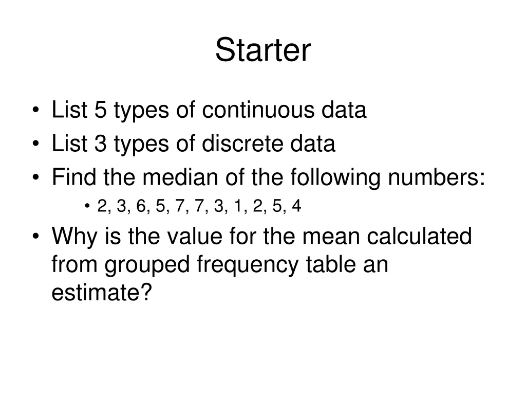
Starter • List 5 types of continuous data • List 3 types of discrete data • Find the median of the following numbers: • 2, 3, 6, 5, 7, 7, 3, 1, 2, 5, 4 • Why is the value for the mean calculated from grouped frequency table an estimate?
Finding the Mean Midpoint t t x f 17 ≤ t < 18 17.5 17.5 x 4 = 70 18 ≤ t < 19 18.5 18.5 x 7 = 129.5 19.5 19.5 x 8 = 156 19 ≤ t < 20 mean = 1247 20 ≤ t < 21 20.5 20.5 x 13 = 266.5 60 21.5 x 12 = 256 21 ≤ t < 22 21.5 = 20.8 (3s.f.) 22.5 22 ≤ t < 23 22.5 x 9 = 202.5 23 ≤ t < 24 23.5 23.5 x 7 = 164.5 Total = 1247
Continuous Data Data that can take any value (within a range) Examples: time, weight, height, etc. You can imagine the class boundaries as fences between a continuous line of possible values 0 2 4 6 8 10 time (for example) These classes would be written as: 0 ≤ t < 2 2 ≤ t < 4 4 ≤ t < 6 6 ≤ t < 8 8 ≤ t < 10 • Each class has: • An upper bound • A lower bound • A class width • A midpoint
Discrete Data Data that can only take certain values Examples: number of people, shoe size. There are only certain values possible. Classes are like a container that hold certain values 0 1 2 3 4 5 6 7 8 9 10 11 n, number of people These classes would be written as: 0 - 1 2 - 3 4 - 5 6 - 7 8 - 9 10 - 11 • Each class has: • An upper bound • A lower bound • A class width • A midpoint
Cumulative Frequency 17 ≤ t < 18 17 ≤ t < 18 18 ≤ t < 19 17 ≤ t < 19 11 19 19 ≤ t < 20 17 ≤ t < 20 32 20 ≤ t < 21 17 ≤ t < 21 21 ≤ t < 22 17 ≤ t < 22 44 53 22 ≤ t < 23 17 ≤ t < 23 60 23 ≤ t < 24 17 ≤ t < 24
Cumulative Frequency Curve f 60 Line is a smooth curve NOT straight lines between each point 50 17 ≤ t < 18 40 17 ≤ t < 19 11 30 19 17 ≤ t < 20 32 17 ≤ t < 21 20 17 ≤ t < 22 44 plot points at the upper limit of each class 53 10 17 ≤ t < 23 60 17 ≤ t < 24 t 17 18 19 20 21 22 23 24
The Median and the Quartiles The median is the middle value. Another way of thinking about it is to consider at what value exactly half of the samples were smaller and half were bigger. We also look at the quartiles: The lower quartile is the value at which 25% of the samples are smaller and 75% are bigger. If we had 60 runners in a race, it would be the time the 15th runner finished, 25% were quicker, 75% were slower. The upper quartile is the value at which 75% of the samples are smaller and 25% are bigger. Again, for 60 runners, it would be the time the 45th person finished. 75% were quicker, 25% were slower. The interquartile range (IQR) = upper quartile – lower quartile = Q3 – Q1 The IQR gives a measure of the spread of the data. Q1 is the first quartile, or the lower quartile Q2 is the second quartile, or the median, m Q3 is the third quartile, or the upper quartile
Finding the median f Median = m or Q2 We find the value of t when f = 30 60 50 Upper quartile = Q3 We find the value of t when f = 45 40 30 Lower quartile = Q1 We find the value of t when f = 15 20 10 t 17 18 19 20 21 22 23 24 Q1 Q2 Q3
Interquartile Range The interquartile range (IQR) = upper quartile – lower quartile = Q3 – Q1 The IQR gives a measure of the spread of the data. The data between Q1 and Q3 is half of the samples. How packed together are these results? The IQR gives us a measure of this. If the IQR is small, the cumulative frequency curve will be steeper in the middle. This means that more samples are nearer to the mean, If the IQR is large, the cumulative frequency curve will not be so steep in the middle. The samples are more spread out.
PRINTABLE SLIDES • Slides after this point have no animation.
Cumulative Frequency 17 ≤ t < 18 17 ≤ t < 18 18 ≤ t < 19 17 ≤ t < 19 11 19 19 ≤ t < 20 17 ≤ t < 20 32 20 ≤ t < 21 17 ≤ t < 21 21 ≤ t < 22 17 ≤ t < 22 44 53 22 ≤ t < 23 17 ≤ t < 23 60 23 ≤ t < 24 17 ≤ t < 24
Cumulative Frequency Curve f 60 Line is a smooth curve NOT straight lines between each point 50 17 ≤ t < 18 40 17 ≤ t < 19 11 30 19 17 ≤ t < 20 32 17 ≤ t < 21 20 17 ≤ t < 22 44 plot points at the upper limit of each class 53 10 17 ≤ t < 23 60 17 ≤ t < 24 t 17 18 19 20 21 22 23 24
The Median and the Quartiles The median is the middle value. Another way of thinking about it is to consider at what value exactly half of the samples were smaller and half were bigger. We also look at the quartiles: The lower quartile is the value at which 25% of the samples are smaller and 75% are bigger. If we had 60 runners in a race, it would be the time the 15th runner finished, 25% were quicker, 75% were slower. The upper quartile is the value at which 75% of the samples are smaller and 25% are bigger. Again, for 60 runners, it would be the time the 45th person finished. 75% were quicker, 25% were slower. The interquartile range (IQR) = upper quartile – lower quartile = Q3 – Q1 The IQR gives a measure of the spread of the data. Q1 is the first quartile, or the lower quartile Q2 is the second quartile, or the median, m Q3 is the third quartile, or the upper quartile
Finding the median f Median = m or Q2 We find the value of t when f = 30 60 50 Upper quartile = Q3 We find the value of t when f = 45 40 30 Lower quartile = Q1 We find the value of t when f = 15 20 10 t 17 18 19 20 21 22 23 24 Q1 Q2 Q3
Interquartile Range The interquartile range (IQR) = upper quartile – lower quartile = Q3 – Q1 The IQR gives a measure of the spread of the data. The data between Q1 and Q3 is half of the samples. How packed together are these results? The IQR gives us a measure of this. If the IQR is small, the cumulative frequency curve will be steeper in the middle. This means that more samples are nearer to the mean, If the IQR is large, the cumulative frequency curve will not be so steep in the middle. The samples are more spread out.