Download
1 / 38
380 likes | 400 Vues
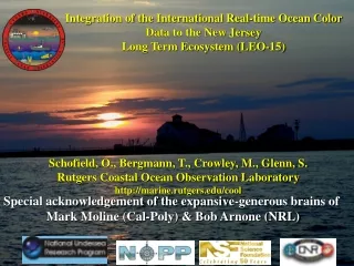
Acknowledging the notable work of Mark Moline and Bob Arnone in integrating real-time ocean color data in New Jersey's Long Term Ecosystem (LEO-15), focusing on bio-optical efforts, phytoplankton pigmentation, chlorophyll distribution, and more. Explore the advancements and challenges in ocean observation for biologists through transects and mooring data analysis.

E N D
Special acknowledgement of the expansive-generous brains of Mark Moline (Cal-Poly) & Bob Arnone (NRL) Integration of the International Real-time Ocean Color Data to the New Jersey Long Term Ecosystem (LEO-15) Schofield, O., Bergmann, T., Crowley, M., Glenn, S. Rutgers Coastal Ocean Observation Laboratory http://marine.rutgers.edu/cool
Goals: Overview of NOPP related bio-optical efforts l What is in the water l Relation to in-water optical properties l Defining the spatial variability l New satellite algorithms and the new platforms l Why ocean observatories are cool for a lowly biologist
Transect Lines & Mooring Locations
Chlorophyll-a July 7 July 16 July 30
16 8 12 mean Chlorophyll a (mg L-1) 8 0 -74.2 -74 4 0 -74.3 -74.2 -74.1 -74 -73.9 -73.8 Longitude Phytoplankton pigmentation determined by High Performance Liquid Chromatography
16 surface 12 bottom 8 Variance in chlorophyll a 4 nearshore 0 -74.3 -74.2 -74.1 -74 -73.9 -73.8 Longitude The Problem
As the Crisis approaches the Nowcast becomes the most important data source, also the time and space scales begin to collapse Forecasts Importance Climatology Nowcast Time Crisis Characterizing the spatial/temporal variability in the coastal zone
High Resolution Maps 0.4 Breve-buster Spectrophotometer 0.3 Absorption (m-1) 0.2 0.1 Day 199 0 Kirkpatrick et al. Applied Optics (In prep.) 400 500 600 700 Wavelength (nm)
Day 195 Day 199
PHYLLS Overflight 8500’ • Hyperspectral Sensor • 1 meter resolution Field Station
Spectra: Red Tide vs. Blue Water ~ 15 m Raw Counts July 22 Red Tide: Run 10 Sequence 6 650 nm band of calibrated data
Radiometers HS-6 AC-9
c a b Ceratium fusus Metridea lucens not shown.
Bioluminescence Potential 1e6 4e10 Photons/sec/ml 0 6 12 Depth (m) 18 24 a 0 1.0 2.0 Distance (km) Distance (km)
1) Prochlorococcus, 2) Green Algae 1) Cryptophytes, 2) Cyanobacteria 1) Diatoms, 2) Dinoflagellates 3)smattering of Coccolithophorrids 12 Chl c Phycobilin 8 Chlorophyll a for different spectral classes of phytoplankton Chl b 4 0 0 5 10 15 20 Total chlorophyll a Discrimination of General Phytoplankton Community Composition From Accessory Carotenoids using ChemTax
1 Closed symbols = cyanobacteria + cryptophytes Green symbols = prasinophytes + chlorophyes + prochlorococcus 0.8 Cryptophytes 0.6 Proportion of Total Chlorophyll a in Chlorophytes or Phycobilin-Algae Cyanobacteria 0.4 Prochlorococcus Green algae 0.2 0 0 0.2 0.4 0.6 0.8 1 1.2 Proportion of Total Chlorophyll a in Chromophytes
Inverting the Signals from Available Instrumentation 1) separate out dissolved and particulate components 2) define the different particulate components diatoms dinoflagellates prymensiophytes prasinophytes euglenophytes Red Peak normalized absorption chlorophytes chrysophytes raphidophytes cryptophytes cyanobacteria 400 500 600 700 Wavlength (nm) Estimated Phytoplankton Absorption Spectra from AC-9 data pink -modeledblue - measured The Good The Bad The Ugly Inverse meters Wavlength (nm)
Derived versus measured phytoplankton community composition 1.5 at depth 1.1 Correlation slope between measured and predicted phytoplankton absorption all 0.7 0.3 surface (n = 68) -0.1 400 450 500 550 600 650 700 Wavelength (nm) 0.8 0.6 R2 0.4 0.2 0 400 450 500 550 600 650 700 Wavelength (nm)
Backscatter - 555nm July 16 July 7
443nm vs. 442nm 0.03 0.02 HS-6 Backscatter (m-1) 0.01 0 0 0.02 0.04 0.06 SeaWiFS Backscatter (m-1)
Correlation coefficients (R2) for in situ backscatter and derived from SeaWiFS satellites Carder Arnone 443nm 490nm 555nm 670nm 443nm 490nm 555nm 670nm 0.63 0.90 442nm ---- ---- ---- ---- ---- ---- 0.55 0.85 488nm ---- ---- ---- ---- ---- ---- July 7 (n=6) 589nm 0.68 0.96 ---- ---- ---- ---- ---- ---- 620nm 0.70 0.96 ---- ---- ---- ---- ---- ---- 0.57 0.57 ---- ---- ---- ---- ---- ---- 442nm 0.64 0.63 488nm ---- ---- ---- ---- ---- ---- July 16 (n=12) 589nm 0.67 0.69 ---- ---- ---- ---- ---- ---- 620nm 0.69 0.74 ---- ---- ---- ---- ---- ---- 442nm 0.65 0.65 ---- ---- ---- ---- ---- ---- 0.62 0.72 488nm ---- ---- ---- ---- ---- ---- July 30 (n=8) 589nm 0.35 0.46 ---- ---- ---- ---- ---- ---- 620nm 0.69 0.76 ---- ---- ---- ---- ---- ----
How does FY1-C Turbidity compare to SeaWiFS chlorophyll-a? FY1-C - October 3, 2000 14:12 GMT (10:12 Local) Turbidity -0.5 -0.25 0 0.25 0.5 0.75 1.0 40N 38N 76W 74W 72W SeaWifs - October 3, 2000 17:32 GMT (1:32 PM Local) Chlorophyll-a (mg/m3) 0.1 0.3 1.1 2.2 2.6 40N 38N 76W 74W 72W
FY1-C vs. SeaWiFS CH9/CH7 3x3 mean filter FY1-C ch9/ch7 August 17, 2000 13:20 GMT SeaWiFS - Chl-a August 16, 2000 17:17 GMT Note: The SeaWiFS values peak at about 2.0 mg/m3. This is well below the values of 5-7 typically seen during upwelling events. If FY1-C can see these values, it will easily see upwelling events.
Time Series Optical Maps 1.0 1 Tidal Cycle Upwelling 6 Absorption at 440 nm (m-1) Depth (m) 0 12 0 30 60 Time (hr) Time Series and Continuous Vicarious Calibration Data
EcoSim 2.0 Model Formulation Air/Sea CO2 Dust Physical Mixing and Advection Light N2 Iron CO2 NH4 NO3 PO4 SiO4 Relict DOM Cocco-litho-phores Benthic Flora Pelagic Diatoms Dino- flagellate Tricho-desmium Synecho- coccus G. breve Excreted DOM Lysed DOM Hetero- Flagellet Viruses Copepod Ciliates Bacteria Sediment Detritus Predator Closure
Conclusions The new ocean color algorithms will provide estimates of the in-water inherent optical properties allowing inversion to material in the water The new international constellation of ocean color satellites will provide an unprecedented temporal picture of the dominant constituents in the coastal ocean These data streams will initialize ocean optical models which will be coupled to the hydrodynamic data-assimilative forecast models Thanks to our NOPP/ONR research partners
1.0 0.0 1.4 1 Absorption-555 Depth (m) 0.6 1.5 0.2 Distance (km) 0 10 Kd (predicted) After Storm (lots nonalgal particles) Upwelling 443 nm 0 Kd (measured) 0 1.5 1.4 Slope of measured & predicted Kd 1 0.6 0.2 443 510 620 443 510 620 412 490 555 670 412 490 555 670 Wavelength (nm) Wavelength (nm) 1 1 0.6 0.6 R2 0.2 0.2 443 510 620 443 510 620 412 490 555 670 412 490 555 670 Wavelength (nm) Wavelength (nm) AC-9 & Default VSF settings
Book from 1954 Observatories
Thermocline Depth and Optics: Particle Max Often at Thermocline ONR HyCODE/COMOP/REA Experiment OSU (Pegau & Boss), Cornell (Philpott) NavAir (Allocca et al.) Passive: Modulation over time of magnitude and shape of the reflectance spectra Active: Changes in Attenuation Slope Profile with Modulated LIDAR Beam Thermocline Fluorescence Depth Range
0.03 0.02 0.01 Offshore Stations Arnone HS-6 Backscatter (m-1) 0 0.03 0.02 0.01 Carder 0 0 0.02 0.04 0.06 SeaWiFS Backscatter (m-1)
For each depth interval light attenuation c(l,t) = a(l,t) + b(l,t) absorption a(l,t) = awater(l) + aphyto(l) + aCDOM(l) + ased(l) scattering b(l,t) = bwater(l) + bphyto(l) + bCDOM(l) + bsed(l) backscattering bb(l,t) = bb,water(l) + bb,phyto(l) + bb,CDOM(l) + bb,sed(l) geometric structure of light md(l) = fxn[b(l,t),c(l ,t), m0(l)] diffuse light attenuation Kd(l) = [a(l,t) + bb(l ,t)]/md(l)] water leaving radiance to a satellite Lu(l) = fxn[a(l,t),b(l ,t), bb(l ,t),Ed(l,t), md(l), md(l), mu(l)] Photon Budgets, Photon Budgets, Photon Budgets! (We can now become optical accountants)
0.03 0.03 Chl-specific Aph676nm 0.02 0.01 0 0 4 0.02 Chromophyte Chl a Chl-specific Aph676nm (m2 mg Chl a-1) 0.01 0 0 2 4 6 8 10 Chlorophyll a (mg L-1) Absorption efficiency decreases (barely) with increase in cell size as predicted by Mie theory
FY1-C - Aug. 27, 2000 13:25 GMT (9:25 AM Local) Channel 4 (AVHRR Ch. 4) 42N 42N 40N 40N 38N 38N 76W 76W 72W 68W 72W 68W AVHRR SST and FY1-C Ch. 4 (FY1-C channel 4 = AVHRR ch 4)