Download

1 / 41
410 likes | 435 Vues
Ratio Games and Designing Experiments. Andy Wang CIS 5930-03 Computer Systems Performance Analysis. Ratio Games. Choosing a base system Using ratio metrics Relative performance enhancement Ratio games with percentages Strategies for winning a ratio game Correct analysis of ratios.

E N D
Ratio GamesandDesigning Experiments Andy Wang CIS 5930-03 Computer Systems Performance Analysis
Ratio Games • Choosing a base system • Using ratio metrics • Relative performance enhancement • Ratio games with percentages • Strategies for winning a ratio game • Correct analysis of ratios
Choosing a Base System • Run workloads on two systems • Normalize performance to chosen system • Take average of ratios • Presto: you control what’s best
Example of Choosinga Base System • (Carefully) selected Ficus results:
Why Does This Work? • Expand the arithmetic:
Using Ratio Metrics • Pick a metric that is itself a ratio • E.g., power = throughput response time • Or cost/performance • Handy because division is “hidden”
Relative Performance Enhancement • Compare systems with incomparable bases • Turn into ratios • Example: compare Ficus 1 vs. 2 replicas with UFS vs. NFS (1 run on chosen day): • “Proves” adding Ficus replica costs less than going from UFS to NFS
Ratio Games with Percentages • Percentages are inherently ratios • But disguised • So great for ratio games • Example: Passing tests • A is worse, but looks better in total line!
More on Percentages • Psychological impact • 1000% sounds bigger than 10-fold (or 11-fold) • Great when both original and final performance are lousy • E.g., salary went from $40 to $80 per week • Small sample sizes generate big lies • Base should be initial, not final value • E.g., price can’t drop 400%
Strategies for Winninga Ratio Game • Can you win? • How to win
Can You Winthe Ratio Game? • If one system is better by all measures, a ratio game won’t work • And selecting the base lets you change the magnitude of the difference • If each system wins on some measures, ratio games might be possible (but no promises) • May have to try all bases
How to WinYour Ratio Game • For LB metrics, use your system as the base • For HB metrics, use the other as a base • If possible, adjust lengths of benchmarks • Elongate when your system performs best • Short when your system is worst • This gives greater weight to your strengths
Correct Analysis of Ratios • Previously covered in Lecture 2 • Generally, harmonic or geometric means are appropriate • Or use only the raw data
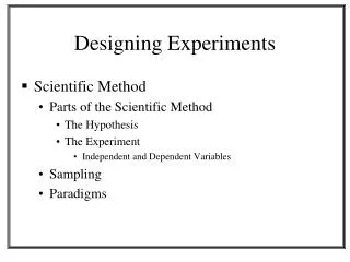
Introduction To Experimental Design • You know your metrics • You know your factors • You know your levels • You’ve got your instrumentation and test loads • Now what?
Goals in Experiment Design • Get maximum info with minimum work • Typically meaning minimum number of experiments • More experiments aren’t better if you’re the one who has to perform them • Well-designed experiments are also easier to analyze
Experimental Replications • System under study will be run with varying levels of different factors, potentially with differing workloads • Run with particular set of levels and other inputs is a replication • Often, need to do multiple replications with each set of levels and other inputs • Usually necessary for statistical validation
Interacting Factors • Some factors have completely independent effects • Double the factor’s level, halve the response, regardless of other factors • But effects of some factors depends on values of others • Called interacting factors • Presence of interacting factors complicates experimental design
The Basic Problemin Designing Experiments • You’ve chosen some number of factors • May or may not interact • How to design experiment that captures full range of levels? • Want minimum amount of work • Which combination or combinations of levels (of factors) do you measure?
Common Mistakesin Experimentation • Ignoring experimental error • Uncontrolled parameters • E.g., CPU voltage scaling • Not isolating effects of different factors • One-factor-at-a-time experimental designs • Interactions ignored • Designs require too many experiments
Types ofExperimental Designs • Simple designs • Full factorial design • Fractional factorial design
Simple Designs • Vary one factor at a time • For k factors with ith factor having ni levels, no. of experiments needed is: • Assumes factors don’t interact • Even then, more effort than required • Don’t use it, usually
Full Factorial Designs • Test every possible combination of factors’ levels • For k factors with ith factor having ni levels: • Captures full information about interaction • But a huge amount of work
Reducing the Work inFull Factorial Designs • Reduce number of levels per factor • Generally good choice • Especially if you know which factors are most important • Use more levels for those • Reduce number of factors • But don’t drop important ones! • Use fractional factorial designs
Fractional Factorial Designs • Only measure some combination of levels of the factors • Must design carefully to best capture any possible interactions • Less work, but more chance of inaccuracy • Especially useful if some factors are known to not interact
2k Factorial Designs • Used to determine effect of k factors • Each with two alternatives or levels • Often used as preliminary to larger performance study • Each factor measured at its maximum and minimum level • Sometimes normal vs. 2x normal, 25% vs. 75% quartiles • Might offer insight on importance and interaction of various factors
Unidirectional Effects • Effects that only increase as level of a factor increases • Or vice versa • If system known to have unidirectional effects, 2k factorial design at minimum and maximum levels is useful • Shows whether factor has significant effect
22 Factorial Designs • Two factors with two levels each • Simplest kind of factorial experiment design • Concepts developed here generalize • Regression can easily be used
22 Factorial Design Example • Consider parallel operating system • Goal is fastest possible completion of a given program • Quality usually expressed as speedup • We’ll use runtime as metric (simpler but equivalent)
Factors and Levelsfor Parallel OS • First factor: number of CPUs • Vary between 8 and 64 • Second factor: use of dynamic load management • Migrates work between nodes as load changes • Other factors possible, but ignore them for now
Defining Variables for22 Factorial OS Example if 8 nodes if 64 nodes if no dynamic load mgmt if dynamic load mgmt
Sample Datafor Parallel OS • Single runs of one benchmark 8 Nodes 64 Nodes NO DLM 820 217 DLM 776 197
Regression Modelfor Example • y = q0 + qAxA + qBxB + qABxAxB • Note that model is nonlinear! 820 = q0 – qA – qB + qAB 217 = q0 + qA – qB – qAB 776 = q0 – qA + qB – qAB 197 = q0 + qA + qB + qAB
Solving the Equations • 4 equations in 4 unknowns • q0 = 502.5 • qA = -295.5 • qB = -16 • qAB = 6 • So y = 502.5 –295.5xA– 16xB + 6xAxB
The Sign Table Method • Write problem in tabular form I A B AB y 1 -1 -1 1 820 1 1 -1 -1 217 1 -1 1 -1 776 1 1 1 1 197 2010 -1182 -64 24 Total 502.5 -295.5 -16 6 Total/4
Allocation of Variationfor 22 Model • Calculate the sample variance of y: • Numerator is SST: total variation SST = 22qA2 + 22qB2 + 22qAB2 • SST explains causes of variation in y
Terms in the SST • 22qA2 is variation explained by effect of A: SSA • 22qB2 is variation explained by effect of B: SSB • 22qAB2 is variation explained by interaction between A and B: SSAB SST = SSA + SSB + SSAB
Variations in Our Example • SST = 350449 • SSA = 349281 • SSB = 1024 • SSAB = 144 • Now easy to calculate fraction of total variation caused by each effect
Fractions of Variation in Our Example • Fraction explained by A is 99.67% • Fraction explained by B is 0.29% • Fraction explained by interaction of A and B is 0.04% • So almost all variation comes from number of nodes • If you want to run faster, apply more nodes, don’t turn on dynamic load management
General 2kFactorial Designs • Used to explain effects of k factors, each with two alternatives or levels • 22 factorial designs are a special case • Same methods extend to more general case • Many more interactions between pairs (and trios, etc.) of factors
Sample 23 Experiment • Sign table A, B, C are binary count; interactions are products of columns: