20. DFS, BFS, Biconnectivity, Digraphs
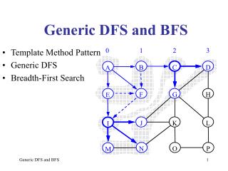
20. DFS, BFS, Biconnectivity, Digraphs. CS 221 West Virginia University. A. B. D. E. C. Depth-First Search. Outline and Reading. Definitions ( § 6.1) Subgraph Connectivity Spanning trees and forests Depth-first search ( § 6.3.1) Algorithm Example Properties Analysis

20. DFS, BFS, Biconnectivity, Digraphs
E N D
Presentation Transcript
20. DFS, BFS, Biconnectivity, Digraphs CS 221 West Virginia University 20.DFS, BFS, Biconnectivity, Digraphs
A B D E C Depth-First Search 20.DFS, BFS, Biconnectivity, Digraphs
Outline and Reading • Definitions (§6.1) • Subgraph • Connectivity • Spanning trees and forests • Depth-first search (§6.3.1) • Algorithm • Example • Properties • Analysis • Applications of DFS (§6.5) • Path finding • Cycle finding 20.DFS, BFS, Biconnectivity, Digraphs
Subgraphs • A subgraph S of a graph G is a graph such that • The vertices of S are a subset of the vertices of G • The edges of S are a subset of the edges of G • A spanning subgraphof G is a subgraph that contains all the vertices of G Subgraph Spanning subgraph 20.DFS, BFS, Biconnectivity, Digraphs
A graph is connected if there is a path between every pair of vertices A connected componentof a graph G is a maximal connected subgraph of G Connectivity Connected graph The vertices inside the yellow oval do not form a connected component. Non connected graph with two connected components 20.DFS, BFS, Biconnectivity, Digraphs
Trees and Forests • A (free) tree is an undirected graph T such that • T is connected • T has no cycles (that is, acyclic) This definition of tree is different from the one of a rooted tree • A forest is an undirected graph without cycles • The connected components of a forest are trees Tree Forest 20.DFS, BFS, Biconnectivity, Digraphs
Spanning Trees and Forests • A spanning treeof a connected graph is a spanning subgraph that is a tree • A spanning tree is not unique unless the graph is a tree • Spanning trees have applications to the design of communication networks • A spanning forestof a graph is a spanning subgraph that is a forest Graph Spanning tree 20.DFS, BFS, Biconnectivity, Digraphs
Depth-first search (DFS) is a general technique for traversing a graph A DFS traversal of a graph G Visits all the vertices and edges of G Determines whether G is connected Computes the connected components of G Computes a spanning forest of G DFS on a graph with n vertices and m edges takes O(n + m ) time DFS can be further extended to solve other graph problems Find and report a path between two given vertices Find a cycle in the graph Depth-first search is to graphs what Euler tour is to binary trees Depth-First Search 20.DFS, BFS, Biconnectivity, Digraphs
DFS Algorithm • The algorithm uses a mechanism for setting and getting “labels” of vertices and edges AlgorithmDFS(G, v) Inputgraph G and a start vertex v of G Outputlabeling of the edges of G in the connected component of v as discovery edges and back edges setLabel(v, VISITED) for all e G.incidentEdges(v) ifgetLabel(e) = UNEXPLORED w G.opposite(v,e) if getLabel(w) = UNEXPLORED setLabel(e, DISCOVERY) DFS(G, w) else setLabel(e, BACK) AlgorithmDFS(G) Inputgraph G Outputlabeling of the edges of G as discovery edges and back edges for all u G.vertices() setLabel(u, UNEXPLORED) for all e G.edges() setLabel(e, UNEXPLORED) for all v G.vertices() ifgetLabel(v) = UNEXPLORED DFS(G, v) 20.DFS, BFS, Biconnectivity, Digraphs
DFS Algorithm If e is an edge between v and w, opposite(v,e) returns w • The algorithm uses a mechanism for setting and getting “labels” of vertices and edges AlgorithmDFS(G, v) Inputgraph G and a start vertex v of G Outputlabeling of the edges of G in the connected component of v as discovery edges and back edges setLabel(v, VISITED) for all e G.incidentEdges(v) ifgetLabel(e) = UNEXPLORED w G.opposite(v,e) if getLabel(w) = UNEXPLORED setLabel(e, DISCOVERY) DFS(G, w) else setLabel(e, BACK) AlgorithmDFS(G) Inputgraph G Outputlabeling of the edges of G as discovery edges and back edges for all u G.vertices() setLabel(u, UNEXPLORED) for all e G.edges() setLabel(e, UNEXPLORED) for all v G.vertices() ifgetLabel(v) = UNEXPLORED DFS(G, v) Under what circumstances will DFS find a vertex that is *not* marked UNEXPLORED? 20.DFS, BFS, Biconnectivity, Digraphs
A B D E C A A B D E B D E C C Example unexplored vertex A visited vertex A unexplored edge discovery edge back edge 20.DFS, BFS, Biconnectivity, Digraphs
A A A B D E B D E B D E C C C A B D E C Example (cont.) 20.DFS, BFS, Biconnectivity, Digraphs
DFS and Maze Traversal • The DFS algorithm is similar to a classic strategy for exploring a maze • We mark each intersection, corner and dead end (vertex) visited • We mark each corridor (edge ) traversed • We keep track of the path back to the entrance (start vertex) by means of a rope (recursion stack) 20.DFS, BFS, Biconnectivity, Digraphs
Property 1 DFS(G, v) visits all the vertices and edges in the connected component of v Property 2 The discovery edges labeled by DFS(G, v) form a spanning tree of the connected component of v A B D E C Properties of DFS DFS(G) visits each connected component. 20.DFS, BFS, Biconnectivity, Digraphs
Setting/getting a vertex/edge label takes O(1) time Each vertex is labeled twice once as UNEXPLORED once as VISITED Each edge is labeled twice once as UNEXPLORED once as DISCOVERY or BACK Method incidentEdges is called once for each vertex DFS runs in O(n + m) time provided the graph is represented by the adjacency list structure Recall that Sv deg(v)= 2m Analysis of DFS 20.DFS, BFS, Biconnectivity, Digraphs
Path Finding AlgorithmpathDFS(G, v, z) setLabel(v, VISITED) S.push(v) if v= z return S.elements() for all e G.incidentEdges(v) ifgetLabel(e) = UNEXPLORED w opposite(v, e) if getLabel(w) = UNEXPLORED setLabel(e, DISCOVERY) S.push(e) pathDFS(G, w, z) S.pop() { e gets popped } else setLabel(e, BACK) S.pop() { v gets popped } • We can specialize the DFS algorithm to find a path between two given vertices u and z using the template method pattern • We call DFS(G, u) with u as the start vertex • We use a stack S to keep track of the path between the start vertex and the current vertex • As soon as destination vertex z is encountered, we return the path as the contents of the stack 20.DFS, BFS, Biconnectivity, Digraphs
AlgorithmDFS(G, v) Inputgraph G and a start vertex v of G Outputlabeling of the edges of G in the connected component of v as discovery edges and back edges setLabel(v, VISITED) for all e G.incidentEdges(v) ifgetLabel(e) = UNEXPLORED w G.opposite(v,e) if getLabel(w) = UNEXPLORED setLabel(e, DISCOVERY) DFS(G, w) else setLabel(e, BACK) AlgorithmpathDFS(G, v, z) setLabel(v, VISITED) S.push(v) if v= z return S.elements() for all e G.incidentEdges(v) ifgetLabel(e) = UNEXPLORED w opposite(v, e) if getLabel(w) = UNEXPLORED setLabel(e, DISCOVERY) S.push(e) pathDFS(G, w, z) S.pop(){ e gets popped } else setLabel(e, BACK) S.pop(){ v gets popped } Comparison of DFS and pathDFS 20.DFS, BFS, Biconnectivity, Digraphs
Cycle Finding AlgorithmcycleDFS(G, v, z) setLabel(v, VISITED) S.push(v) for all e G.incidentEdges(v) ifgetLabel(e) = UNEXPLORED w opposite(v,e) S.push(e) if getLabel(w) = UNEXPLORED setLabel(e, DISCOVERY) pathDFS(G, w, z) S.pop() else C new empty stack repeat o S.pop() C.push(o) until o= w return C.elements() S.pop() • We can specialize the DFS algorithm to find a simple cycle using the template method pattern • We use a stack S to keep track of the path between the start vertex and the current vertex • As soon as a back edge (v, w) is encountered, we return the cycle as the portion of the stack from the top to vertex w What other value can getLabel(e) have? 20.DFS, BFS, Biconnectivity, Digraphs
Cycle Finding AlgorithmcycleDFS(G, v, z) setLabel(v, VISITED) S.push(v) for all e G.incidentEdges(v) ifgetLabel(e) = UNEXPLORED w opposite(v,e) S.push(e) if getLabel(w) = UNEXPLORED setLabel(e, DISCOVERY) pathDFS(G, w, z) S.pop() else C new empty stack repeat o S.pop() C.push(o) until o= w return C.elements() S.pop() • We can specialize the DFS algorithm to find a simple cycle using the template method pattern • We use a stack S to keep track of the path between the start vertex and the current vertex • As soon as a back edge (v, w) is encountered, we return the cycle as the portion of the stack from the top to vertex w What other value can getLabel(e) have? BACK ! 20.DFS, BFS, Biconnectivity, Digraphs
A B D E C Cycle Finding AlgorithmcycleDFS(G, v, z) setLabel(v, VISITED) S.push(v) for all e G.incidentEdges(v) ifgetLabel(e) = UNEXPLORED w opposite(v,e) S.push(e) if getLabel(w) = UNEXPLORED setLabel(e, DISCOVERY) pathDFS(G, w, z) S.pop() else C new empty stack repeat o S.pop() C.push(o) until o= w return C.elements() S.pop() • We can specialize the DFS algorithm to find a simple cycle using the template method pattern • We use a stack S to keep track of the path between the start vertex and the current vertex • As soon as a back edge (v, w) is encountered, we return the cycle as the portion of the stack from the top to vertex w 20.DFS, BFS, Biconnectivity, Digraphs
AlgorithmDFS(G, v) Inputgraph G and a start vertex v of G Outputlabeling of the edges of G in the connected component of v as discovery edges and back edges setLabel(v, VISITED) for all e G.incidentEdges(v) ifgetLabel(e) = UNEXPLORED w G.opposite(v,e) if getLabel(w) = UNEXPLORED setLabel(e, DISCOVERY) DFS(G, w) else setLabel(e, BACK) AlgorithmcycleDFS(G, v, z) setLabel(v, VISITED) S.push(v) for all e G.incidentEdges(v) ifgetLabel(e) = UNEXPLORED w opposite(v,e) S.push(e) if getLabel(w) = UNEXPLORED setLabel(e, DISCOVERY) pathDFS(G, w,z) S.pop() else C new empty stack repeat o S.pop() C.push(o) until o= w return C.elements() S.pop() Comparison of DFS and cycleDFS 20.DFS, BFS, Biconnectivity, Digraphs
AlgorithmpathDFS(G, v, z) setLabel(v, VISITED) S.push(v) if v= z return S.elements() for all e G.incidentEdges(v) ifgetLabel(e) = UNEXPLORED w opposite(v, e) if getLabel(w) = UNEXPLORED setLabel(e, DISCOVERY) S.push(e) pathDFS(G, w, z) S.pop(){ e gets popped } else setLabel(e, BACK) S.pop() { v gets popped } AlgorithmcycleDFS(G, v, z) setLabel(v, VISITED) S.push(v) for all e G.incidentEdges(v) ifgetLabel(e) = UNEXPLORED w opposite(v,e) S.push(e) if getLabel(w) = UNEXPLORED setLabel(e, DISCOVERY) pathDFS(G, w, z) S.pop() else C new empty stack repeat o S.pop() C.push(o) until o= w return C.elements() S.pop() Comparison of pathDFS and cycleDFS 20.DFS, BFS, Biconnectivity, Digraphs
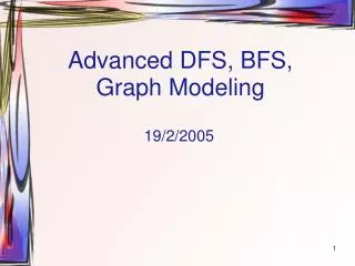
L0 A L1 B C D L2 E F Breadth-First Search 20.DFS, BFS, Biconnectivity, Digraphs
L0 A L1 B C D L2 E F A B D E C Visual Comparison of DFS and BFS BFS DFS 20.DFS, BFS, Biconnectivity, Digraphs
Outline and Reading • Breadth-first search (§6.3.3) • Algorithm • Example • Properties • Analysis • Applications • DFS vs. BFS (§6.3.3) • Comparison of applications • Comparison of edge labels 20.DFS, BFS, Biconnectivity, Digraphs
Breadth-first search (BFS) is a general technique for traversing a graph A BFS traversal of a graph G Visits all the vertices and edges of G Determines whether G is connected Computes the connected components of G Computes a spanning forest of G BFS on a graph with n vertices and m edges takes O(n + m ) time BFS can be further extended to solve other graph problems Find and report a path with the minimum number of edges between two given vertices Find a simple cycle, if there is one Breadth-First Search 20.DFS, BFS, Biconnectivity, Digraphs
DFS can be further extended to solve other graph problems Find and report a path between two given vertices Find a cycle in the graph BFS can be further extended to solve other graph problems Find and report a path with the minimum number of edges between two given vertices Find a simple cycle, if there is one [see next slide for review of simple cycle definition] Comparison of DFS and BFS extensions 20.DFS, BFS, Biconnectivity, Digraphs
Terminology (review) Cycle circular sequence of alternating vertices and edges each edge is preceded and followed by its endpoints Simple cycle cycle such that all its vertices and edges are distinct Examples C1=(V,b,X,g,Y,f,W,c,U,a,) is a simple cycle C2=(U,c,W,e,X,g,Y,f,W,d,V,a,) is a cycle that is not simple V a b d U X Z C2 h e C1 c W g f Y 19. Graphs 20.DFS, BFS, Biconnectivity, Digraphs 28
BFS Algorithm AlgorithmBFS(G, s) L0new empty sequence L0.insertLast(s) setLabel(s, VISITED) i 0 while Li.isEmpty() Li +1new empty sequence for all v Li.elements() for all e G.incidentEdges(v) ifgetLabel(e) = UNEXPLORED w opposite(v,e) if getLabel(w) = UNEXPLORED setLabel(e, DISCOVERY) setLabel(w, VISITED) Li +1.insertLast(w) else setLabel(e, CROSS) i i +1 • The algorithm uses a mechanism for setting and getting “labels” of vertices and edges AlgorithmBFS(G) Inputgraph G Outputlabeling of the edges and partition of the vertices of G for all u G.vertices() setLabel(u, UNEXPLORED) for all e G.edges() setLabel(e, UNEXPLORED) for all v G.vertices() ifgetLabel(v) = UNEXPLORED BFS(G, v) 20.DFS, BFS, Biconnectivity, Digraphs
L0 A L1 B C D E F Example unexplored vertex A visited vertex A unexplored edge discovery edge cross edge L0 L0 A A L1 L1 B C D B C D E F E F 20.DFS, BFS, Biconnectivity, Digraphs
L0 L0 A A L1 L1 B C D B C D L2 E F E F L0 L0 A A L1 L1 B C D B C D L2 L2 E F E F Example (cont.) 20.DFS, BFS, Biconnectivity, Digraphs
L0 L0 A A L1 L1 B C D B C D L2 L2 E F E F Example (cont.) L0 A L1 B C D L2 E F 20.DFS, BFS, Biconnectivity, Digraphs
Comparison of DFS and BFS AlgorithmDFS(G, v) Inputgraph G and a start vertex v of G Outputlabeling of the edges of G in the connected component of v as discovery edges and back edges setLabel(v, VISITED) for all e G.incidentEdges(v) ifgetLabel(e) = UNEXPLORED w G.opposite(v,e) if getLabel(w) = UNEXPLORED setLabel(e, DISCOVERY) DFS(G, w) else setLabel(e, BACK) AlgorithmBFS(G, s) L0new empty sequence L0.insertLast(s) setLabel(s, VISITED) i 0 while Li.isEmpty() Li +1new empty sequence for all v Li.elements() for all e G.incidentEdges(v) ifgetLabel(e) = UNEXPLORED w opposite(v,e) if getLabel(w) = UNEXPLORED setLabel(e, DISCOVERY) setLabel(w, VISITED) Li +1.insertLast(w) else setLabel(e, CROSS) i i +1 20.DFS, BFS, Biconnectivity, Digraphs
Notation Gs: connected component of s Property 1 BFS(G, s) visits all the vertices and edges of Gs Property 2 The discovery edges labeled by BFS(G, s) form a spanning tree Ts of Gs Property 3 For each vertex v in Li The path of Ts from s to v has i edges Every path from s to v in Gshas at least i edges Properties A B C D E F L0 A L1 B C D L2 E F 20.DFS, BFS, Biconnectivity, Digraphs
Setting/getting a vertex/edge label takes O(1) time Each vertex is labeled twice once as UNEXPLORED once as VISITED Each edge is labeled twice once as UNEXPLORED once as DISCOVERY or CROSS Each vertex is inserted once into a sequence Li Method incidentEdges is called once for each vertex BFS runs in O(n + m) time provided the graph is represented by the adjacency list structure Recall that Sv deg(v)= 2m Analysis 20.DFS, BFS, Biconnectivity, Digraphs
Applications • Using the template method pattern, we can specialize the BFS traversal of a graph Gto solve the following problems in O(n + m) time • Compute the connected components of G • Compute a spanning forest of G • Find a simple cycle in G, or report that G is a forest • Given two vertices of G, find a path in G between them with the minimum number of edges, or report that no such path exists 20.DFS, BFS, Biconnectivity, Digraphs
L0 A L1 B C D L2 E F DFS vs. BFS A B C D E F DFS BFS 20.DFS, BFS, Biconnectivity, Digraphs
Back edge(v,w) w is an ancestor of v in the tree of discovery edges Cross edge(v,w) w is in the same level as v or in the next level in the tree of discovery edges L0 A L1 B C D L2 E F DFS vs. BFS (cont.) A B C D E F DFS BFS 20.DFS, BFS, Biconnectivity, Digraphs
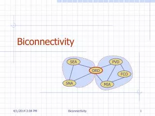
Biconnectivity SEA PVD ORD FCO SNA MIA 20.DFS, BFS, Biconnectivity, Digraphs
Outline and Reading • Definitions (§6.3.2) • Separation vertices and edges • Biconnected graph • Biconnected components • Equivalence classes • Linked edges and link components • Algorithms (§6.3.2) • Auxiliary graph • Proxy graph 20.DFS, BFS, Biconnectivity, Digraphs
Definitions Let G be a connected graph A separation edge of G is an edge whose removal disconnects G A separation vertex of G is a vertex whose removal disconnects G Applications Separation edges and vertices represent single points of failure in a network and are critical to the operation of the network Example DFW, LGA and LAX are separation vertices (DFW,LAX) is a separation edge Separation Edges and Vertices ORD PVD SFO LGA HNL LAX DFW MIA 20.DFS, BFS, Biconnectivity, Digraphs
Comment on Terminology • I’m accustomed to the term “cut” rather than “separation.” 20.DFS, BFS, Biconnectivity, Digraphs
Biconnected Graph • Equivalent definitions of a biconnected graph G • Graph G has no separation edges and no separation vertices • For any two vertices u and v of G,there are two disjoint simple paths between u and v (i.e., two simple paths between u and v that share no other vertices or edges) • For any two vertices u and v of G, there is a simple cycle containing u and v • Example PVD ORD SFO LGA HNL LAX DFW MIA 20.DFS, BFS, Biconnectivity, Digraphs
Biconnected Components • Biconnected component of a graph G • A maximal biconnected subgraph of G, or • A subgraph consisting of a separation edge of G and its end vertices • Interaction of biconnected components • An edge belongs to exactly one biconnected component • A nonseparation vertex belongs to exactly one biconnected component • A separation vertex belongs to two or more biconnected components • Example of a graph with four biconnected components ORD PVD SFO LGA RDU HNL LAX DFW MIA 20.DFS, BFS, Biconnectivity, Digraphs
Equivalence Classes • Given a set S, a relation R on S is a set of ordered pairs of elements of S, i.e., R is a subset of SS • An equivalence relation R on S satisfies the following properties Reflexive: (x,x)R Symmetric: (x,y)R (y,x)R Transitive: (x,y)R (y,z)R (x,z)R • An equivalence relation R on S induces a partition of the elements of S into equivalence classes • Example (connectivity relation among the vertices of a graph): • Let V be the set of vertices of a graph G • Define the relationC = {(v,w) VV such that G has a path from v to w} • Relation C is an equivalence relation • The equivalence classes of relation C are the vertices in each connected component of graph G 20.DFS, BFS, Biconnectivity, Digraphs
i g e b a d j f c Link Relation • Edges e and f of connected graph Gare linked if • e = f, or • G has a simple cycle containing e and f Theorem: The link relation on the edges of a graph is an equivalence relation Proof Sketch: • The reflexive and symmetric properties follow from the definition • For the transitive property, consider two simple cycles sharing an edge Equivalence classes of linked edges: {a} {b, c, d, e, f} {g, i, j} i g e b a d j f c 20.DFS, BFS, Biconnectivity, Digraphs
The link components of a connected graph G are the equivalence classes of edges with respect to the link relation A biconnected component of G is the subgraph of G induced by an equivalence class of linked edges A separation edge is a single-element equivalence class of linked edges A separation vertex has incident edges in at least two distinct equivalence classes of linked edge Link Components ORD PVD SFO LGA RDU HNL LAX DFW MIA 20.DFS, BFS, Biconnectivity, Digraphs
Auxiliary Graph h g i e b • Auxiliary graph B for a connected graph G • Associated with a DFS traversal of G • The vertices of B are the edges of G • For each back edge e of G, B has edges (e,f1), (e,f2) , …, (e,fk),where f1, f2, …, fk are the discovery edges of G that form a simple cycle with e • Its connected components correspond to the the link components of G i j d c f a DFS on graph G g e i h b f j d c a Auxiliary graph B 20.DFS, BFS, Biconnectivity, Digraphs
Auxiliary Graph (cont.) • In the worst case, the number of edges of the auxiliary graph is proportional to nm DFS on graph G Auxiliary graph B 20.DFS, BFS, Biconnectivity, Digraphs
Proxy Graph h g AlgorithmproxyGraph(G) Inputconnectedgraph GOutputproxy graph F for GFempty graph DFS(G, s) { s is any vertex of G} for all discovery edges e of G F.insertVertex(e) setLabel(e, UNLINKED) for all vertices v of G in DFS visit order for all back edges e= (u,v) F.insertVertex(e) repeat fdiscovery edge with dest. u F.insertEdge(e,f,) if fgetLabel(f) =UNLINKED setLabel(f, LINKED) uorigin of edge f else uv{ ends the loop } until u=v returnF i e b i j d c f a DFS on graph G g e i h b f j d c a Proxy graph F 20.DFS, BFS, Biconnectivity, Digraphs