Resolution: Implications in Refinement
Resolution: Implications in Refinement. Swanand Gore & Gerard Kleywegt May 6 th 2010, 12-1 pm. Macromolecular Crystallography Course. Outline. Intuitive idea of resolution – why higher order diffraction is better. Parameters, model, observations, refinement – more data is better.

Resolution: Implications in Refinement
E N D
Presentation Transcript
Resolution: Implications in Refinement Swanand Gore & Gerard Kleywegt May 6th 2010, 12-1 pm Macromolecular Crystallography Course
Outline • Intuitive idea of resolution – why higher order diffraction is better. • Parameters, model, observations, refinement – more data is better. • Observations, parameters, over-fitting in crystallographic refinement. • Features that can be modeled at various resolutions. • Refinement practices at low and high resolution.
Idealized diffraction in 1D h3 h2 h1 -h1 -h2 -h3 • Images scanned from David Blow’s book
Idealized diffraction in 1D h3 h2 • Assuming: • B = 0 • Occupancy = 1 • Uniform scattering power in all directions. • Phase angles = 0 h1 -h1 -h2 -h3 Increasing resolution • Images scanned from David Blow’s book
Idealized diffraction in 1D • Higher order diffraction • Higher Fourier coefficients • Higher frequency wave in real space • Sharper signal • Greater resolution • Images scanned from David Blow’s book
What separation can be resolved? O O • Nominal resolution • The h-th order diffracted wave samples the lattice at interval of a/h. • a/h is the crystallographic resolution which is routinely quoted. • In tetragonal cell abc, diffraction hkl comes from planes separated by • √[ (a/h)2 + (b/k)2 + (c/l)2 ] • For tetragonal cell 100, 95, 90, and highest order diffraction 50, 52, 48, resolution is ~3.29. • For non-orthogonal axes, corrections apply. • Resolution intuitively means the least distance between objects below which they cannot be distinguished apart. • For 3D crystallography, it is ~0.92*dmin, almost same as nominal. blob • Images from B. Rupp’s book • Image from Gerard’s ppt.
Atomic scatterers in 1D Resolution Filter Peaks get sharper as higher resolution Fourier coefficients are included. Fourier Coefficients & Phases C O C C O O • Images fromB. Rupp’s book
Occupancy and B factors Peaks get broader due to larger B factors and shorter due to lower occupancy. • Images from B. Rupp’s book
Data truncation Happens naturally due to B factors. Truncated data leads to incomplete reverse FT, causes ripples. Ripples around heavy atoms can ‘drown’ nearby lighter atoms. Ripples can seem to originate from real atoms. N’s at 0.5 occupancy? O at 0.5 occupancy? • Images from B. Rupp’s book
Diffracting duck in 2D • Leaving out higher order diffraction data will reduce the detail retrieved through reverse transform. • Leaving out lower resolution data will blur the boundaries. • Randomly absent data is not too problematic for maps. • Doesn’t matter if Rfree set is / not used in map calc? • Images from Kevin Cowtan’s website.
Make everything as simple as possible,but not simpler….. ρx = 1/V ΣFh exp (-2πih.x + iφh) • Fh exp(iφh) =V Σfioi exp(2πih.x) exp (-Bi sin2θ/λ2) Noise. Errors in data collection. Static, dynamic disorder. Estimate phases. Model xyz, B, o. Model solvent. ….. • Images from B. Rupp’s book
Choosing resolution cutoff • B factors and scattering factors impose a natural cutoff on what can be observed. • Reliability of measurement is indicated by S/N ratio and completeness • Signal to noise ratio • A low SNR does not matter too much if proper maximum likelihood target is used to weigh in error estimates. • High <I/σ(I)> matters when collecting data for phasing. • Completeness • Low completeness in highest resolution shell does not confer a level of detail to the map as implied by nominal resolution • Effective resolution = dmin . C-1/3 • Randomly or systematically missing data creates undesirable effects in reverse FT. • Completeness > 0.95 • Number of reflections increases as cube of nominal resolution. • 2/3z π VUC / dmin3 • Not unique due to centro-symmetry and spacegroup symmetry • Images from B. Rupp’s book
Model and refinement • Model is defined as a set of parameters and a set of functions over parameters, designed to explain observations • Refinement • Is an algorithmic process of fitting a model to explain observations, by assigning optimal values to parameters. • Reduces the differences between observations and model-calculated values of observations • A linear model in 2D consists of 2 parameters • Y = mX + c • Some models are more accurate than others, depending on quality of refinement. • Refinement is necessary when observations contain errors and there are enough observations to refine the parameters. Observations Well-refined model Ill-refined model m 1 c
Model and refinement • A linear model in 2D • consists of 2 parameters : Y = mX + c • 1 observation, howsoever accurate, is not sufficient if model has 2 parameters • Under-determined, over-fitted model • Many models can be imagined • 2 distinct accurate observations are sufficient to determine the linear model • Well-determined model • 3 accurate observations over-determine the model • But observations generally contain random error! Greater number of observations lead to error cancellation and more accurate model • Model with too few params can lead to under-fitting • Model with too many params can lead to over-fitting • Fitting to error too! • Quality of modelling • Choice of model (linear, quadratic, higher polynomial?) • Quality of refinement (R value) • Images from B. Rupp’s book
M1 Model and refinement M2 • In presence of errors, refinement quality does not indicate model quality • Well-refined model is of bad quality if it was fitted to erroneous observations. • Hence, observations not subject to refinement are required to assess the accuracy. • R and “free” R • M1: 0.2, 0.3 • M2: 0.2, 0.4 • M1 better than M2 • Free R and data/param ratio helps in comparing models with different number of parameters • MA: 0.2, 0.3. d/p = 15/2 = 7.5 • Under-fit • MB: 0.1, 0.2. d/p = 15/3 = 5 • optimal • MC: 0.01, 0.25. d/p = 15/10 = 1.5 • Overfitting = Low d/p, high Rfree MC MA MB Occham’s valley • Images from B. Rupp’s book
A crystallographic model • Biochemical entities • Biopolymers • polypeptides, polynucleotides, carbohydrates • Small-molecule ligands (ions, organic) • Crystallographic additives, e.g. GOL, PEG • Physiologically relevant, e.g. heme, ions • Synthesized molecules, e.g. a drug candidate • Solvent • Coordinates, Displacement • Unique x,y,z • Partial, multiple, absent (occupancy) • Isotropic or anisotropic B factors • TLS approximation • Crystallographic etc. • Cell, symmetry, NCS • Bulk solvent correction (Ksol, Bsol) • 3hbq images made with pymol. • http://www.cgl.ucsf.edu/chimera/feature_highlights/ellipsoids.png • B factor putty from Antonyuket al. 10.1073/pnas.0809170106 • www.ruppweb.org/xray/tutorial/Crystal_sym.htm
Quick note on NCS, TLS • Non-crystallograpic symmetry • Molecule/s -> ASU -> locally-related ASUs -> Unitcell -> Crystal • Sometimes ASU can consist of multiple, nearly identical subunits. • The transformation operator between subunits is local and distinct from space-group operators. • Subunits need not be identical because they are in different environments, differences do not indicate problems! • This additional symmetry can be used in refinement (restraints, constraints) and validation. • Translation-libration-screw • Overall anisotropy = lattice disorder + inter-molecular motions + intra-molecular rigid body motions within molecule + atomic anisotropy • Paradigm shift from atom-level anisotropy modelling to anisotropic movements of rigid bodies • 1d: a point (3) through which rotation axis (2) will pass + ratio (1) of rotation to translation on that axis = 6 • 2d: 2 points + 2 ratios + 2 orthogonal axes (3) + 2 more ratios = 13 • 3d: 3 points + 3 ratios + 3 orthogonal axes (3) + 6 more screws = 20(ish) • TLS group granularity can range from full domain to sidechain • Images from Rupp book and Martyn Winn ppt
Counting parameters 1clm, calmodulin, 1.8Å 1132 protein atoms + 4 Ca + 71 waters = 4828 xyzB #unique reflections = 10610 Data / params = 2.2 • Average-case parameters • Per atom 4 params • 3 params for coordinates • 1 param for isotropic B factor • No hydrogens, 1 water per residue • 8 atoms per residue • N * 8 * 4 = 32 N • Increasing the parameters • 6 params per atom for anisotropic B factor (>2x) • Refining occupancy (1.25x) or multiple occupancy • Hydrogens modeled explicitly (8 per residue) (2x) • Multiple models (M x) • Reducing parameters • 20 params per TLS group • 5 groups: 20 * 5 groups of 40 res each = 100 • => 32 * 200 to 100 (1/64 x for 200 res protein) • Strict NCS (1/n x for n-fold) 1exr, calmodulin, 1Å 1467 protein atoms with alt conf + 5 Ca + 178 waters 9900 anisotropic B + 316 occupancy = 15166 params #unique reflections = 77150 Data / params = 4.6 1h6v , 3Å 6 TLS groups = 120 params 22514 protein atoms + 552 ligand atoms + 9 waters xyzB = 92300 (residual) #unique reflections = 69328 (5% free) d/p = 69328/92300 = 0.7 • Restraint counts taken from: http://ccp4wiki.org/~ccp4wiki/wiki/images/9/9f/Winn_prague09_data_parameters.pdf
Data to parameters ratio • r = (number of unique reflections) / (number of parameters) • Graph for a calmodulin 1up5, ~2500 atoms, xyzB • r < 1, i.e. under-determined for dmin < 2.5Å • Reflections-based refinement is possible only for r > 10, i.e. resolution approaching 1Å! • But most PDB entries have r ~ 2-5 • There must be more observations provided to refinement than only the reflections • Reflections = observations specific to a particular MX experiment • But there are other more general observations applicable to any MX refinement • Covalent geometry, steric clashes, …. (Graph by KonradHinsen, 2008) • Image from B. Rupp’s book
Observations to parameters ratio • Observations = reflections + constraints and restraints based on well-known features of macromolecules • o/p > d/p • Tricky to estimate the difference due to dependences, but generally sufficient to make refinement possible • 1exr: 1Å, 22732 restraints • Bonds, angles, planarity, chirality… • o/p = (22732 + 77150) / 15166 = 6.1 > 4.6 = d/p Hangman CONvict = CONstraint Bungee jumper RElaxation = REstraint Energy length • Images from Gerard’s slides • Restraint counts taken from: http://ccp4wiki.org/~ccp4wiki/wiki/images/9/9f/Winn_prague09_data_parameters.pdf
Observations to parameters ratio • o/p > d/p for 1h6v at 3Å • Restraints (including NCS) = 209378 • o/p = (209378+69328)/92300 = 3 • d/p = 0.7 < 3 = o/p • 2 components of refinement residuals • Data-based • Changes model (xyzB..) to reduce Fo ~ Fc • Knowledge-based • Changes model (xyz) to take values of geometric features towards idealized values • Qtot = wxQx + Qgeom • Small wx: greater stress on geometric correctness • Low resolution, low d/p • Large wx: model deviation from ideal geometry • High resolution, high d/p • Restraint counts taken from: http://ccp4wiki.org/~ccp4wiki/wiki/images/9/9f/Winn_prague09_data_parameters.pdf
Greater d/p => more detail(given decent phases) 0.95Å • Image from http://www.crystal.uwa.edu.au/px/alice/projects/SCOA_atomic.html, 1mxt • Images from Rupp’s book
Lower d/p => lower detaildecent phases often not available 2g34, 5Å 1z56, 3.9Å • Pics of 2g34, 1z56 with coot using EDS maps
Lower d/p => lower detail 2bf1, 4Å • Pics of 2bf1 with coot using EDS maps
All resolutions not equal… • From Gerard’s slides and Phil Evans
Levels of detail interpretableat various resolutions Orbitals and bonds (beyond 1Å)! • From David Blow’s book
Rules of thumb at all resolutions for model-building and refinement • Start with few parameters and slowly enrich the model • Be very conservative till a majority of backbone is identified and produces stable refinement • Prioritize: Backbone > side-chains > small-mols > waters • Be aware of prevalent modeling practices at your resolution • Whole model contributes to quality of region of interest. • Use similar structures for comparison and copying. • Use quality criteria often.
Low resolution refinement • Low resolution structures offer great biological insights. • Mainly for complexes e.g. 70S ribosome at 7Å, SIV gp120 envelope glycoprotein at 4Å • Large complexes generally diffract to lower resolution. • Components may have physiologically relevant conformations only in complexed states. • High impact • In absence of better resolution, low resolution data must be used. • Low resolution does not have to mean low quality! • Basic guidelines for model building and refinement. • Low d/p => Be cautious of biasing the model • Make extensive use of information in addition to reflections • Use as few parameters as possible • Increase params only when confident • Images from Karmali et al. ActaCryst. 2009.
Low resolution refinement • Build model with fewer parameters • Mainchain-only model • Constrain B factor values to be isotropic and constant. • Full occupancies only. • TLS to model anisotropic motions of rigid domains. • Strictly constrained or restrained NCS to reduce params many-fold • No waters or small molecules, use only ‘bulk solvent’
Low resolution refinement • Model cautiously • Initial tracing • Build regions that are likely to be seen clearly • Good packing, low B factors, bulky group, electron-rich groups • core, mainchain, helices, big sidechains, bases, phosphates • Sequence registry • Beware of register and topology errors • Guess sequence register from bulky sidechains • Extend the register by trial and error • Check sequence register with a homologous structure • Truncate to Gly wherever unsure of residue identity • From Gerard’s slides
Low resolution refinement • Try copying fragments from other high resolution structures when there is clear homology • Treat ligands extra-carefully • Copy high-quality observed conformation or predicted low energy conformation • Restrain tightly unless there is density and other clues to deviate • Axel T. Brunger et al. 2009. ActaCryst D 65 128–133 X-ray structure determination at low resolution.
Low resolution refinementdensity modification tools • Expected solvent density • define solvent boundary • followed by solvent flattening / flipping, histogram matching • Images B. Rupp’s book and from ActaCryst. (2003). D59, 1881-1890. The phase problem. G. Taylor • Brunger 2006, Low resolution crystallography. ActaCryst. • https://wasatch.biochem.utah.edu/chris/tutorial/Density_Modification.pdf a ppt on DM
Low resolution refinementdensity modification • Averaging maps of NCS-restrained copies • Image from B. Rupp’s Brook. • unger 2006, Low resolution crystallography. ActaCryst. • https://wasatch.biochem.utah.edu/chris/tutorial/Density_Modification.pdf a ppt on DM
Low resolution refinementdensity modification • B-factor sharpening • High-resolution reflections get attenuated most by B factors • Application of negative B factors can artificially up-weigh high-res terms to obtain greater detailed but possibly noisier map • Brunger 2006, Low resolution crystallography. ActaCryst. • https://wasatch.biochem.utah.edu/chris/tutorial/Density_Modification.pdf a ppt on DM
Low resolution refinement • Refinement techniques • Rigid body refinement • A fragment is constrained to be internally rigid, has only 6 degrees of freedom • B factor is isotropic and constant • Powerful first step of refinement needing only low resolution data • Arbitrary rigid fragments (high quality helices, high-resolution domain structures) can be optimized for location and orientation relative to each other to yield better phases and maps • Torsion angle refinement • Bonds, angles, chirality, planarity not variables, only torsion angles are refined • Protein is divided into rigid subgroups to sample thoroughly a limited conformational space • Higher radius of convergence, reduced overfitting • Image from Schwieters, C.D. & Clore, G.M. (2001) Internal coordinates for molecular dynamics and minimization in structure determination and refinement. J. Magn. Reson. 152, 288-302 • Nice tutorial at http://speedy.st-and.ac.uk/~naismith/workshop/torsion.pdf • See Axel Brunger’s papers on torsion angle refinement
Low resolution refinement • Solving multiple times • Try to automate as much as possible the process of model building and refinement, and then repeat it • Consensus substructures are more reliable, average them • Regions with differences are unreliable, remove them • Gives an idea of precision • Gradual increase in number of parameters • Mainchain -> bulky sidechains -> sequence register -> other sidechains • Finally known small mol binders with known binding site can be modelled if reasonable density appears • Validation • Keep track of Ramachandran and sidechainsrotamers • Remove unlikely parts of mainchain and sidechain • Do not restrain Rama distribution or sidechains to rotamers during refinement, it may give false validation results • Read what others are doing for low resolution • e.g. Axel Brunger’s literature, CCP4 & phenix tools, CCP4bb • Images from wikipedia and Furnham et al. Structure 2006.
High resolution refinement • High resolution structures provide atomic insights • Packing, binding • Flexibility • Enzyme mechanisms • Hydration • Basic guidelines for model building and refinement • High d/p => Be cautious of under-fitting! • Make greater use of data than in low res case • Make as detailed a model as possible, esp of interesting regions • Check all empty density critically
High resolution refinement • Allow model to deviate from geometry when data is strong • Weight on xray term can be slowly increased to reveal any unusual geometry without risking model bias • Use automation to fit biopolymers • Trace secondary structure automatically, in coot or with phenix tools • Trace mainchain and build sidechains using programs, e.g. with buccaneer, warpNtrace, Rapper • Do this multiple times to identify regions requiring manual attention • Validation tools: can they indicate the information content of macromolecular crystal structures? EJ Dodson et al. Volume 6, Issue 6, 1998, 685-690. • Image from Terwillinger et al. papers in ActaCryst D on automatic chain tracing.
High resolution refinement • Explain all unoccupied density • Is it due to ligands? • Build expected ligands (including MX additives) • Search unexpected small-mols • E.g. coot or phenixligand tools • Is it due to multi-conformer sidechains? • Is it water? • Images from B. Rupp’s book and Terwillinger et al. ActaCryst. 2005.
High resolution refinement • Build waters • Peak-pick semi-automatically to form a reasonable hydration network with sidechains • Model hydrogens • When difference density is visible • Image from B. Rupp’s book • Atomic resolution crystallography reveals how changes in pH shape the protein microenvironment. Lyubimov et al. Nature Chemical Biology 2, 259 - 264 (2006)
High resolution refinement • Verify correct sidechain orientations of NQH • Manually or automatically flip NQH sidechains to improve h-bonding • Model more sidechain conformations if necessary • Use non-standard atomic scattering models • At subatomic resolution, model electron density with nonsphericalmultipolar model, or model bonds as scatterers • Image from B. Rupp’s book • Afonine et al. ActaCryst. (2007). D63, 1194–1197 • Jelsch et al. PNAS 2000 97 7 3171.
High resolution refinement • Even in high res, maintain order of adding detail to avoid overfitting • bb > sc > ligand • Anisotropy, multiconformers, waters, hydrogens • Invest more parameters around the regions of interest • multi-conformers • Anisotropy • waters near active site • Possibility of multiple ligands • Releasing constraints / restraints • Image from AntonyukS V et al. PNAS 2005;102:12041-12046 • Image from David Blow’s book.
Summary • Resolution is the least distance between Bragg planes with observable reflection. Two atoms closer than resolution cannot be observed distinctly using data at that resolution. • Resolution dictates the detail revealed by electron density maps. • Low resolution => low detail • High resolution => high detail • Parameters in the model must be chosen to suit the resolution. • Over-fitting can be detected using Rfree and data to parameter ratio. • Knowledge-based constraints and restraints augment experimental data to make refinement possible. • Geometric target is weighted more than crystallographic data at low resolution. Model is allowed to diverge from ideal geometry at high resolution. • Greater detail should be modelled at higher resolution to make best use of data.
Acknowledgements • Alejandro & IPMont MX organizers • SameerVelankar, JawaharSwaminathan (EBI) • Online resources • Kevin Cowtan • Rupp web • Randy Read’s course • Various papers and images therefrom • Martyn Winn’s ppt at on data to params • Books • David Blow • Alex McPherson • Bernhard Rupp