
Optimal Location and Pricing Strategy for Beverage Delivery in Kreis Coesfeld
Solve a realistic location problem for a beverage delivery service in Kreis Coesfeld, considering costs, demand, and distance to cities. Determine the optimal location and pricing simultaneously using mathematical calculations. Find the best balance between rent, transport costs, and variable expenses for maximizing profit. Utilize the Pythagorean theorem to calculate distances and linear price functions at different locations. Enhance profitability by adjusting prices based on competition and distance.

Optimal Location and Pricing Strategy for Beverage Delivery in Kreis Coesfeld
E N D
Presentation Transcript
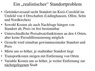
Ein „realistisches“ Standortproblem • Getränkeversand sucht Standort im Kreis Coesfeld im Umfeld von 4 Ortschaften (Lüdinghausen, Olfen, Selm und Nordkirchen) • Sowohl Kosten als auch Nachfrage hängen von Standort ab, Preis ist frei bestimmbar • Unterschiedliche Preisabsatzfunktionen an den 4 Orten, aber keine Preisdifferenzierung möglich • Gesucht wird simultan gewinnmaximaler Standort und Preis • Miete um so höher, je stadtnäher Standort liegt • Transportkosten steigen mit Entfernung von Orten • Variable Kosten um so höher, je weiter Entfernung zur nächstgelegenen Stadt
Errechnen von Entfernungen im xy-Koordinatensystem LH yl NK uls Es gilt nach dem Satz des Pythargoras: uls2 = (yl – ys)2 + xl –xs)2 S yn d.h. uls = [(yl – ys)2 + xl –xs)2]0,5 Olf Selm xl xn
An jedem Ort i gilt (unterschiedliche) lineare Preisabsatzfunktion (abhängig auch von Konkurrenz): pi p = ai – bi*Xi => Xi = (ai - p)/bi Gesamterlös E = p * (X1 + X1 ...) Xi Kges = Bodenkosten (Miete) + Transportkosten + variable Kosten Bodenkosten = B + B1/(1+u1) + B2/(1+u2) + ... Preis auf dem Land Zuschläge für Stadtnähe, abhängig von Stadtgröße (Bi) und Entfernung Transportkosten T = T1 + T2 + ... mit Ti = t * Xi * ui
Variable Kosten Kv (Arbeit, Vorprodukte) steigen mit wachsender Entfernung vom nächstgelegenen Ort: Kv = X * k * [1 + z * min(u1; u2 ; u3 ...)] Gesamt- absatz Variable Kosten in der Stadt Zuschlag wegen Stadtferne Zu maximieren ist Gewinn G = E – Kges Variable sind der Standort (Koordinaten xs und ys) sowie der (für alle Orte einheitliche) Absatzpreis (Transportkosten trägt der Getränkeversand) Lösung auf numerischem Wege (siehe Excel-Datei)