Angle-domain Wave-equation Reflection Traveltime Inversion
340 likes | 528 Vues
Angle-domain Wave-equation Reflection Traveltime Inversion. Sanzong Zhang, Yi Luo and Gerard Schuster ( 1) KAUST, ( 2) Aramco. 1. 2 . 1. Outline. Introduction Theory and method Numerical examples Conclusions. Outline. Introduction Theory and method

Angle-domain Wave-equation Reflection Traveltime Inversion
E N D
Presentation Transcript
Angle-domain Wave-equation Reflection Traveltime Inversion SanzongZhang, Yi Luo and Gerard Schuster (1) KAUST, (2) Aramco 1 2 1
Outline • Introduction • Theory and method • Numerical examples • Conclusions
Outline • Introduction • Theory and method • Numerical examples • Conclusions
Velocity Inversion Methods Ray-based tomography Data space Wave-equ. Reflection traveltimeinversion (Tomography) Full Waveform inversion Inversion Ray-based MVA Wave-equ. Reflection traveltimeinversion Image space (MVA) Wave-equ.MVA
Problem • The waveform (image) residual is highly nonlinear with respect to velocity change. 2 - e = Model Parameter Pred. data – Obs. data • The traveltime misfit function enjoys a somewhat linear relationship with velocity change.
Angle-domain Wave-equation Reflection TraveltimeInversion • Traveltime inversion without high-frequency approximation • Misfit function somewhat linear with respect to velocity perturbation. • Wave-equation inversion less sensitive to amplitude • Multi-arrival traveltimeinversion • Beam-based reflection traveltime inversion
Outline • Introduction • Theory and method • Numerical examples • Conclusions
Wave-equationTransmission Traveltime Inversion 1). Observed data 5 0 Time (s) 2). Calculated data Time (s) 0 5 3). 1.5 0 -1.5 Lag time (s) 4). Smear time delay along wavepath
Angle-domain Wave-equation Reflection Traveltime Inversion Suboffset-domain crosscorrelation function : ) g s x+h x-h : : time shift x
Angle-domain Crosscorrelation • Angle-domain CIG decomposition (slant stack ): angle-domain suboffset-domain • Angle-domain crosscorrelation function : )
Angle-domain Crosscorrelation: physical meaning ) ) ) Local plane wave Local plane wave • Angle-domain crosscorrelation is the crosscorrelation • between downgoing and upgoing beams with a certain angle. • The time delay for multi-arrivals is available in angle • -domain crosscorrelation function .
Angle-domain Wave-equation Reflection Traveltime Inversion Objective function: Velocity update: (x)=(x) + (x) Gradient function: Traveltimewavepath
TraveltimeWavepath • Angle-domain time delay • Angle-domain connective function • Traveltimewavepath
Transforming CSG Data Xwell Trans. Data reflection transmission transmission = + Src-side XwellData source Redatuming source Rec-side XwellData Observed data Redatuming data
Workflow • Forward propagate source to trial image points and get downgoing beams • Backward propagate observed reflection data from geophonsesto trial image points , and get upgoing beams • Crosscorrelatedowngoing beam and upgoing beam, and pick angle-domain time delay • Smear time dealy along wavepath to update velocity model
Outline • Introduction • Theory and method • Numerical examples • Simple Salt Model • Sigsbee Salt Model • Conclusions
Simple Salt Model (c) Initial Velocity Model (d) RTM image (a) True velocity model 5 0 0 0 z (km) V(km/s) z (km) z (km) 1 4 4 4 x (km) 8 x (km) 8 x (km) 8 0 0 0 (b) CSG 0 t (s) 0 x (km) 8 5
Angle-domain Crosscorrelation (a) Initial Velocity Model (b) Angle-domain Crosscorrelation 0 z (km) 4 8 x (km) 0 (c) Angle-domain Crosscorrelation time delay curvature reflection angle
Inversion Result (a) Initial velocity model 0 5 z (km) Velocity(km/s) 1 4 8 x (km) 0 (b) Inverted velocity model 0 z (km) 8 0 x (km) 4
Inversion Result (a) RTM image 0 z (km) 4 8 x (km) 0 (b) RTM image 0 z (km) 0 x (km) 8 4
Outline • Introduction • Theory and method • Numerical examples • Simple Salt Model • Sigsbee Salt Model • Conclusions
Sigsbee Model (b) Initial velocity model (a) True velocity model 0 0 0 z(km) z(km) z(km) Vinitial = 0.85 Vtrue 6 6 6 0 0 0 12 12 12 x(km) x(km) x(km) (c) RTM image 4.5 Velocity (km/s) 1.5
Initial Velocity Model 0 z(km) CIG Crosscorrelation Semblance 0 6 -0.2 0 12 x(km) 0 z(km) z(km) 6 0.2 6 -50° +50° -0.04 0.04 -50° +50°
Initial Velocity Model 0 z(km) CIG Crosscorrelation Semblance 0 6 -0.2 0 12 x(km) 0 z(km) z(km) 6 0.2 6 -50° +50° -0.04 0.04 -50° +50°
Initial Velocity Model 0 z(km) CIG Crosscorrelation Semblance 0 6 -0.2 0 12 x(km) 0 z(km) z(km) 6 0.2 6 -50° +50° -0.04 0.04 -50° +50°
Inverted Velocity Model 0 z(km) CIG Crosscorrelation Semblance 0 6 -0.2 0 12 x(km) 0 z(km) z(km) 6 0.2 6 -50° +50° -0.04 0.04 -50° +50°
Inverted Velocity Model 0 z(km) CIG Semblance Crosscorrelation 0 6 -0.2 0 12 x(km) 0 z(km) z(km) 6 0.2 6 -50° +50° -0.04 0.04 -50° +50°
Inverted Velocity Model 0 z(km) CIG Crosscorrelation Semblance 0 6 -0.2 0 12 x(km) 0 z(km) z(km) 6 0.2 6 -50° +50° -0.04 0.04 -50° +50°
RTM Image 0 0 z(km) z(km) 6 6 (a) RTM image using initial velocity (b) RTM image using inverted model 12 x(km) 0 0 x(km) 12
Outline • Introduction • Theory and method • Numerical examples • Conclusions
Velocity Inversion Methods Ray-based tomography Data space Wave-equ. traveltime inversion (Tomography) Full Wavform inversion Inversion Ray-based MVA Wave-equ. traveltime inversion Image space (MVA) Wave-equ.MVA
Angle-domain Wave-equation Reflection TraveltimeInversion • Traveltime inversion without high-frequency approximation • Misfit function somewhat linear with respect to velocity perturbation. • Wave-equation inversion less sensitive to amplitude • Multi-arrival traveltimeinversion • Beam-based reflection traveltime inversion