
Mucin
SCFM. MOPS. Egg yolk. DNA. BSA. MDTA. Mucin. Supplementary Figure 1. 1 H NMR spectra generated for SCFM media and selected constituents. pH 7.0. pH 6.8. pH 6.4. pH 6.2. pH 6.0. pH 5.8. pH 5.6. pH 5.4.

Mucin
E N D
Presentation Transcript
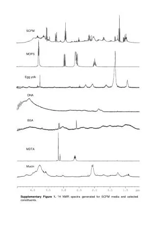
SCFM MOPS Egg yolk DNA BSA MDTA Mucin Supplementary Figure 1. 1H NMR spectra generated for SCFM media and selected constituents.
pH 7.0 pH 6.8 pH 6.4 pH 6.2 pH 6.0 pH 5.8 pH 5.6 pH 5.4 Supplementary Figure 2. 1H NMR spectra generated for MOPS buffer in 10% D2O at various pH
A B Supplementary Figure 3. Correction of peak shifting using Correlation Optimized Warping (COW). Correction works well for the region containing between 4.20 and 3.60 ppm (A), however alignment of the multiple peaks between 2.30 and 2.00 ppm is unsuccessful (B).
Supplementary Figure 4. Loadings plot, corresponding to the PCA scores scatter plot shown in Figure 2, identifies points in the NMR spectra that align with either PC1 or PC2
A B Supplementary Figure 5. Leave-one-out cross-validation (LOOCV) output files for the comparisons of SCFM (blue) and putative Clusters I (A) and IIa (B) (both red). From top left to bottom right: scores plots showing good separation between classes; back-scaled loadings plots showing 1H resonance frequencies that discriminate between the two classes under comparison; histograms showing number of principal components used to separate the classes; prediction residual error sum of squares(PRESS) indicating low within-sample variation; Q2 value histogram comparing random class assignment (grey) and the actual class assignment (blue); comparison of model predicted for the sample classification as compared to the actual class.
A B Supplementary Figure 6. Leave-one-out cross-validation (LOOCV) output files for the comparisons of SCFM (blue) and putative Clusters IIb (A) and IIc (B) (both red). From top left to bottom right: scores plots showing good separation between classes; back-scaled loadings plots showing 1H resonance frequencies that discriminate between the two classes under comparison; histograms showing number of principal components used to separate the classes; prediction residual error sum of squares(PRESS) indicating low within-sample variation; Q2 value histogram comparing random class assignment (grey) and the actual class assignment (blue); comparison of model predicted for the sample classification as compared to the actual class.
A B Supplementary Figure 7. Leave-one-out cross-validation (LOOCV) output files for the comparisons of Cluster IIc and either putative Clusters IIa (A) or IIb (B) in a putative four cluster model. Scores for Cluster IIc shown in red (A) and then blue (B). From top left to bottom right: scores plots showing good separation between classes; back-scaled loadings plots showing 1H resonance frequencies that discriminate between the two classes under comparison; histograms showing number of principal components used to separate the classes; prediction residual error sum of squares(PRESS) indicating low within-sample variation; Q2 value histogram comparing random class assignment (grey) and the actual class assignment (blue); comparison of model predicted for the sample classification as compared to the actual class.
A B Supplementary Figure 8. Leave-one-out cross-validation (LOOCV) output files for the comparisons of Cluster IIa (blue) and Cluster IIb (red) in a 3 (A) or 4 (B). From top left to bottom right: scores plots showing good separation between classes; back-scaled loadings plots showing 1H resonance frequencies that discriminate between the two classes under comparison; histograms showing number of principal components used to separate the classes; prediction residual error sum of squares(PRESS) indicating low within-sample variation; Q2 value histogram comparing random class assignment (grey) and the actual class assignment (blue); comparison of model predicted for the sample classification as compared to the actual class.
A B Supplementary Figure 9. Leave-one-out cross-validation (LOOCV) output files for the comparisons of Cluster I (blue) and Cluster IIb (red) in a 3 (A) or 4 (B) class model. From top left to bottom right: scores plots showing good separation between classes; back-scaled loadings plots showing 1H resonance frequencies that discriminate between the two classes under comparison; histograms showing number of principal components used to separate the classes; prediction residual error sum of squares(PRESS) indicating low within-sample variation; Q2 value histogram comparing random class assignment (grey) and the actual class assignment (blue); comparison of model predicted for the sample classification as compared to the actual class.
* A * * * * B * Supplementary Figure 10. Box plots comparing FEV1 (A) and spent culture pH (B) for each of the clusters in the three cluster model; * p < 0.05.
Supplementary Figure 11. RAPD profiles generated from each of the P. aeruginosa clinical isolates. A – profiles generated using primer ERIC2, B - profiles generated using primer ERIC1. The size marker ladder shown is MassRuler Express (Fermentas, UK).
Supplementary Table 1. Relationships between the sample characteristics and strain cluster membership. Assessment of significance was performed using a one-way ANOVA unless stated (#) whereby a Kruskal-Wallis test was used. Asterisk denotes significant (p < 0.05). R2 indicates the amount of variance in the characteristics accounted for by the cluster membership.