Modeling a Microclimate within Vegetation
Modeling a Microclimate within Vegetation. Hisashi Hiraoka Academic Center for Computing and Media Studies Kyoto University. NATO ASI, KIEV 2004. 1. Outline. ◊ introduction • background • review • objective ◊ explanation of our microclimate model ◊ validation of the model

Modeling a Microclimate within Vegetation
E N D
Presentation Transcript
Modeling a Microclimate within Vegetation Hisashi Hiraoka Academic Center for Computing and Media Studies Kyoto University NATO ASI, KIEV 2004 1
Outline ◊ introduction • background • review • objective ◊ explanation of our microclimate model ◊ validation of the model ◊ application of the model to a single tree • the environment around the tree • the heat budget within the tree NATO ASI, KIEV 2004 2
Introduction NATO ASI, KIEV 2004 3
Background of this study numerically investigatng the effect of vegetation on a heat load of a building, thermal comfort, an urban thermal environment and the like. • trees beside a house (heat load) • roof garden (heat load, thermal comfort) • garden (microclimate, thermal comfort) • street trees (thermal comfort) • park (microclimate, thermal comfort) • wooded area in a city (urban thermal environment) • woods (effect on urban thermal environment) • forest (effect on urban thermal environment) NATO ASI, KIEV 2004 4
Review of researches • Waggoner and Reifsnyder (1968) • Lemon et al. (1971) • Goudriaan (1977) • Norman (1979) • Horie (1981) • Meyers and Paw U (1987) • Naot and Mahrer (1989) • Kanda and Hino (1990) Necessary sub-models * turbulence model * radiation transfer model* stomatal conductance model* model for water uptake of root* model for heat and water diffusion in soil ◊ soil respiration model◊ root respiration model NATO ASI, KIEV 2004 5
Problems of the above models • These models are not completely applicable to 3dim. • Short wave radiation is not separated into PAR and the other. Objective of this study • Proposing a model for simulating a microclimate within three-dimensional vegetation • Examining the validity of the model by comparing with measurement • Applying the model to a single model tree and investigating the microclimate produced by the tree NATO ASI, KIEV 2004 6
Microclimate Model for Vegetation NATO ASI, KIEV 2004 7
Outline of our microclimate model • turbulence model the present model [Table 1] • Ross’s radiation transfer model assumption 1: A scattering characteristic of a single leaf is of Lambertian type. Diffusion Approximation : surface harmonic series expanded up to the first-order • stomatal conductance model by Collatz et al. (1991) assumption 2: Vegetation is adequately supplied with water from soil. NATO ASI, KIEV 2004 8
Formulation of turbulence model Basic equations are first ensemble-averaged and then spatially averaged. (2) The turbulence equations for dispersive componentand real turbulent component are derived from thebasic equation and the averaged equations. (3) These two kinds of equations are combined intothe turbulence equation. (4) And the unknown quantities are modeled by the semi-empirical closure technique. NATO ASI, KIEV 2004 9
Definition of spatial average: : filter function [formulas] (1) (2) : the averaged volume , where : the fluid volume in : the i-th component of the velocity on leaf surface G =1 in this study. NATO ASI, KIEV 2004 10
An example of a filtering function (1 dimension) NATO ASI, KIEV 2004 11
Symbols : instantaneous value of : ensemble mean of : spatial mean of : time fluctuation, or deviation from ensemble mean : deviation from spatial mean NATO ASI, KIEV 2004 12
Table 1 Turbulence model for moist air within vegetation (1) (2) transpiration photosynthesis drag force (3) sensible heat heat transfer due to photosynthesis (4) (5) photosynthesis photosynthesis : represents the modeled terms. (6) drag force (7) : represents the vegetation terms which are originally expressed as leaf-surface integral except that in the e equation. These terms are derived analytically from the basic equations by averaging spatially. NATO ASI, KIEV 2004 13
The vegetation terms (1): leaf-surface integral , NATO ASI, KIEV 2004 14
The vegetation term in the k equation (2): NATO ASI, KIEV 2004 15
The equation of k’: : Real turbulent component buoyancy production from mean shear flow production from dispersive component viscous dissipation molecular diffusion turbulent diffusion surface integral term NATO ASI, KIEV 2004 16
The equation of k”: : dispersive component of turbulent energy production by drag force viscous dissipation buoyancy production from mean shear flow dissipation toward real turbulent component molecular diffusion turbulent diffusion NATO ASI, KIEV 2004 17
The equation of turbulent energy k: • production from dispersive component • dissipation toward real turbulent component NATO ASI, KIEV 2004 18
NATO ASI, KIEV 2004 The e equation : production from mean shear flow buoyancy vortex stretching molecular dissipation production from dispersive component turbulent diffusion turbulent diffusion molecular diffusion production from dispersive component production from mean flow 19
The modeled terms: Modeling [Reynolds stress] [other turbulent fluxes] [the vegetation term in the e equation] dimensional analysis according to Launder production from dispersive component NATO ASI, KIEV 2004 20
Table 2 The balances of heat, vapor and CO2 on leaves [a] Heat exchange between leaves and the surrounding air (1) short-wave radiations absorbed by leaves net long- wave radiation transpiration (latent heat) photosynthesis (sensible heat) sensible heat transfer between leaves and air [b] The balance of water vapor flux on leaves (2) transpiration rate [c] Net photosynthetic rate stomatal conductance (3) net photosynthetic rate NATO ASI, KIEV 2004 21
Ross’s radiation transfer models (Short wave radiation) (Long wave radiation) [symbols] : radiance , : direction of radiance : distribution function of foliage area orientation : scattering function of leaf, : emissivity of leaf : leaf area density , : leaf temperature : direction of leaf surface, : inner product NATO ASI, KIEV 2004 22
Outline of stomatal conductance model by Collatz et al. Ball’s empirical equation (1) The value 1.6 means the ratio in molecular diffusivity of CO2 to H2O. (2) simplified Farquhar’s photosynthesis model (3) • The photosynthesis model was made on the basis of Rubisco enzyme reaction in Calvin cycle of C3 plant. • Refer to the paper by Collatz et al. (1991) for the details. NATO ASI, KIEV 2004 23
Verification of the Model NATO ASI, KIEV 2004 24
Verification of the present model The measurement by Naot and Mahrer (1989) • plant: cotton field (1.4m high, 1-dimension) • location: Gilgal (25Km north of the Dead Sea), Israel • period: August 18 - 20, 1987 (3 days) • weather: fair during the period Comparison with the measurement • physical quantities compared with the measurement (1) wind velocity at the height of 1.4m, and 2.5m (2) air temperature at the height of 1.4m (3) net radiant flux NATO ASI, KIEV 2004 25
the model by Svensson and Haggkvist (or Yamada): the present model: Fig. 1 Optimization of the coefficient cep in the e equation NATO ASI, KIEV 2004 26
Fig. 2 Measured and calculated diurnal changes in wind velocity NATO ASI, KIEV 2004 27
Fig. 3 Measured and calculated diurnal changes in air temperature at the height of 1.4m NATO ASI, KIEV 2004 28
Fig. 4 Measured and calculated diurnal changes in net radiant flux NATO ASI, KIEV 2004 29
Application of the Model to a Single Model Tree NATO ASI, KIEV 2004 30
Application of the model to a single tree (1) Outline of computation • computational domain: 48m(x-axis)X30m(y-axis)X30m(z-axis) • tree: 6m cubical foliage whose center is at a point(15m, 15m, 7m) leaf area density: 1[m2/m3] distribution function of foliage area orientation: uniform leaf transmissivity: 0.1(PAR), 0.5(NIR) <- short wave reflectivity: 0.1(PAR), 0.4(NIR) <- short wave emissivity: 0.9 <- long wave • sun: the solar altitude (h): 60 [degree] the atmospheric transmittance (P): 0.8 • the diffused solar radiation: <- Berlarge’s equation • PAR conversion factor at h=60: 0.425(direct), 0.7(diffuse) <- Ross • the downward atmospheric radiation <- Brunt’s equation • calculation method: FDM, SMAC, QUICK, Adams-Bashforth <- Bouguer’s equation NATO ASI, KIEV 2004 31
Application of the model to a single tree (2) Results of computation: the microclimate produced by the tree the atmospheric conditions: • wind velocity: 2 [m/s] • air temperature: 20 [C] • relative humidity: 40 [%] • CO2 mole fraction: 340 [mmol/mol] Figures: • Fig. 5 wind velocity vectors • Fig. 6 distribution of air temperature • Fig. 7 distribution of specific humidity • Fig. 8 distribution of CO2 mole fraction All figures are illustrated as graphs in (x-z) cross section through the center of the tree. NATO ASI, KIEV 2004 32
[m/s] Fig. 5 Wind velocity vectors NATO ASI, KIEV 2004 33
Wind Velocity Vectors NATO ASI, KIEV 2004 34
Wind Velocity Vectors NATO ASI, KIEV 2004 35
Fig. 6 Distribution of air temperature NATO ASI, KIEV 2004 36
Fig. 7 Distribution of specific humidity NATO ASI, KIEV 2004 37
Fig.8 Distribution of CO2 mole fraction NATO ASI, KIEV 2004 38
Pressure Distribution NATO ASI, KIEV 2004 39
Application of the model to a single tree (3-1) Results of computation: the heat budget within foliage Figures: • Fig. 9 PAR absorbed by leaves • Fig. 10 NIR absorbed by leaves • Fig. 11 net long wave radiation • Fig. 12 distribution of latent heat • Fig. 13 distribution of sensible heat • Fig. 14 distribution of sensible heat of water vapor due to transpiration All figures are illustrated as graphs in (x-z) cross section through the center of the tree. NATO ASI, KIEV 2004 40
Fig. 9 PAR absorbed by leaves NATO ASI, KIEV 2004 41
Fig. 10 NIR absorbed by leaves NATO ASI, KIEV 2004 42
Fig. 11 Net long wave radiation NATO ASI, KIEV 2004 43
Fig. 12 Distribution of latent heat NATO ASI, KIEV 2004 44
Fig. 13 Distribution of sensible heat NATO ASI, KIEV 2004 45
Fig. 14 Distribution of sensible heat of water vapor due to transpiration NATO ASI, KIEV 2004 46
Application of the model to a single tree (3-2) Summary of the heat budget within foliage • A great deal of the short wave radiation absorbed by leaves is released through latent heat due to transpiration. • Long wave radiation is not negligible. • Air sensible heat (that is, heat convection term) is much less than latent heat. • Sensible heat of water vapor due to transpiration is negligible. NATO ASI, KIEV 2004 47
Application of the model to a single tree (4) Results of computation: the others Figures: • Fig. 15 transpiration rate within foliage • Fig. 16 net CO2 assimilation rate • Fig. 17 stomatal conductance • Fig. 18 leaf temperature These figures are illustrated as graphs in a (x-z) cross section through the center of the tree. NATO ASI, KIEV 2004 48
Fig. 15 Transpiration rate within foliage NATO ASI, KIEV 2004 49
Fig. 16 Net CO2 assimilation rate NATO ASI, KIEV 2004 50