MAP Estimation Algorithms in
MAP Estimation Algorithms in. Computer Vision - Part I. M. Pawan Kumar, University of Oxford Pushmeet Kohli, Microsoft Research. Aim of the Tutorial. Description of some successful algorithms Computational issues Enough details to implement Some proofs will be skipped :-(


MAP Estimation Algorithms in
E N D
Presentation Transcript
MAP Estimation Algorithms in Computer Vision - Part I M. Pawan Kumar, University of Oxford Pushmeet Kohli, Microsoft Research
Aim of the Tutorial • Description of some successful algorithms • Computational issues • Enough details to implement • Some proofs will be skipped :-( • But references to them will be given :-)
A Vision Application Binary Image Segmentation How ? Cost function Models our knowledge about natural images Optimize cost function to obtain the segmentation
A Vision Application Binary Image Segmentation Graph G = (V,E) Object - white, Background - green/grey Each vertex corresponds to a pixel Edges define a 4-neighbourhood grid graph Assign a label to each vertex from L = {obj,bkg}
A Vision Application Binary Image Segmentation Graph G = (V,E) Object - white, Background - green/grey Per Vertex Cost Cost of a labelling f : V L Cost of label ‘bkg’ high Cost of label ‘obj’ low
A Vision Application Binary Image Segmentation Graph G = (V,E) Object - white, Background - green/grey Per Vertex Cost Cost of a labelling f : V L Cost of label ‘bkg’ low Cost of label ‘obj’ high UNARY COST
A Vision Application Binary Image Segmentation Graph G = (V,E) Object - white, Background - green/grey Per Edge Cost Cost of a labelling f : V L Cost of same label low Cost of different labels high
A Vision Application Binary Image Segmentation Graph G = (V,E) Object - white, Background - green/grey Per Edge Cost Cost of a labelling f : V L Cost of same label high PAIRWISE COST Cost of different labels low
A Vision Application Binary Image Segmentation Graph G = (V,E) Object - white, Background - green/grey Problem: Find the labelling with minimum cost f*
A Vision Application Binary Image Segmentation Graph G = (V,E) Problem: Find the labelling with minimum cost f*
Another Vision Application Object Detection using Parts-based Models How ? Once again, by defining a good cost function
Another Vision Application Object Detection using Parts-based Models H T 1 L1 L2 L3 L4 Graph G = (V,E) Each vertex corresponds to a part - ‘Head’, ‘Torso’, ‘Legs’ Edges define a TREE Assign a label to each vertex from L = {positions}
Another Vision Application Object Detection using Parts-based Models H T 2 L1 L2 L3 L4 Graph G = (V,E) Each vertex corresponds to a part - ‘Head’, ‘Torso’, ‘Legs’ Edges define a TREE Assign a label to each vertex from L = {positions}
Another Vision Application Object Detection using Parts-based Models H T 3 L1 L2 L3 L4 Graph G = (V,E) Each vertex corresponds to a part - ‘Head’, ‘Torso’, ‘Legs’ Edges define a TREE Assign a label to each vertex from L = {positions}
Another Vision Application Object Detection using Parts-based Models H T 3 L1 L2 L3 L4 Graph G = (V,E) Cost of a labelling f : V L Unary cost : How well does part match image patch? Pairwise cost : Encourages valid configurations Find best labelling f*
Another Vision Application Object Detection using Parts-based Models H T 3 L1 L2 L3 L4 Graph G = (V,E) Cost of a labelling f : V L Unary cost : How well does part match image patch? Pairwise cost : Encourages valid configurations Find best labelling f*
Yet Another Vision Application Stereo Correspondence Disparity Map How ? Minimizing a cost function
Yet Another Vision Application Stereo Correspondence Graph G = (V,E) Vertex corresponds to a pixel Edges define grid graph L = {disparities}
Yet Another Vision Application Stereo Correspondence Cost of labelling f : Unary cost + Pairwise Cost Find minimum cost f*
The General Problem 1 2 b c Graph G = ( V, E ) 1 Discrete label set L = {1,2,…,h} a d 3 Assign a label to each vertex f: V L f e 2 2 Cost of a labelling Q(f) Unary Cost Pairwise Cost Find f* = arg min Q(f)
Outline • Problem Formulation • Energy Function • MAP Estimation • Computing min-marginals • Reparameterization • Belief Propagation • Tree-reweighted Message Passing
Energy Function Label l1 Label l0 Vb Vc Vd Va Db Dc Dd Da Random Variables V= {Va, Vb, ….} Labels L= {l0, l1, ….} Data D Labelling f: {a, b, …. } {0,1, …}
Energy Function 6 3 2 4 Label l1 Label l0 5 3 7 2 Vb Vc Vd Va Db Dc Dd Da Easy to minimize Q(f) = ∑a a;f(a) Neighbourhood Unary Potential
Energy Function 6 3 2 4 Label l1 Label l0 5 3 7 2 Vb Vc Vd Va Db Dc Dd Da E : (a,b) E iff Va and Vb are neighbours E = { (a,b) , (b,c) , (c,d) }
Energy Function 0 6 1 3 2 0 4 Label l1 1 2 3 4 1 1 Label l0 1 0 5 0 3 7 2 Vb Vc Vd Va Db Dc Dd Da Pairwise Potential Q(f) = ∑a a;f(a) +∑(a,b) ab;f(a)f(b)
Energy Function 0 6 1 3 2 0 4 Label l1 1 2 3 4 1 1 Label l0 1 0 5 0 3 7 2 Vb Vc Vd Va Db Dc Dd Da Q(f; ) = ∑a a;f(a) +∑(a,b) ab;f(a)f(b) Parameter
Outline • Problem Formulation • Energy Function • MAP Estimation • Computing min-marginals • Reparameterization • Belief Propagation • Tree-reweighted Message Passing
MAP Estimation 0 6 1 3 2 0 4 Label l1 1 2 3 4 1 1 Label l0 1 0 5 0 3 7 2 Vb Vc Vd Va Q(f; ) = ∑a a;f(a) + ∑(a,b) ab;f(a)f(b)
MAP Estimation 0 6 1 3 2 0 4 Label l1 1 2 3 4 1 1 Label l0 1 0 5 0 3 7 2 Vb Vc Vd Va Q(f; ) = ∑a a;f(a) + ∑(a,b) ab;f(a)f(b) 2 + 1 + 2 + 1 + 3 + 1 + 3 = 13
MAP Estimation 0 6 1 3 2 0 4 Label l1 1 2 3 4 1 1 Label l0 1 0 5 0 3 7 2 Vb Vc Vd Va Q(f; ) = ∑a a;f(a) + ∑(a,b) ab;f(a)f(b)
MAP Estimation 0 6 1 3 2 0 4 Label l1 1 2 3 4 1 1 Label l0 1 0 5 0 3 7 2 Vb Vc Vd Va Q(f; ) = ∑a a;f(a) + ∑(a,b) ab;f(a)f(b) 5 + 1 + 4 + 0 + 6 + 4 + 7 = 27
MAP Estimation 0 6 1 3 2 0 4 Label l1 1 2 3 4 1 1 Label l0 1 0 5 0 3 7 2 Vb Vc Vd Va q* = min Q(f; ) = Q(f*; ) Q(f; ) = ∑a a;f(a) + ∑(a,b) ab;f(a)f(b) f* = arg min Q(f; )
MAP Estimation f* = {1, 0, 0, 1} 16 possible labellings q* = 13
Computational Complexity Segmentation 2|V| |V| = number of pixels ≈ 320 * 480 = 153600
Computational Complexity Detection |L||V| |L| = number of pixels ≈ 153600
Computational Complexity Stereo |L||V| |V| = number of pixels ≈ 153600 Can we do better than brute-force? MAP Estimation is NP-hard !!
Computational Complexity Stereo |L||V| |V| = number of pixels ≈ 153600 Exact algorithms do exist for special cases Good approximate algorithms for general case But first … two important definitions
Outline • Problem Formulation • Energy Function • MAP Estimation • Computing min-marginals • Reparameterization • Belief Propagation • Tree-reweighted Message Passing
Min-Marginals 0 6 1 3 2 0 4 Label l1 1 2 3 4 1 1 Label l0 1 0 5 0 3 7 2 Vb Vc Vd Va Not a marginal (no summation) such that f(a) = i f* = arg min Q(f; ) Min-marginal qa;i
Min-Marginals qa;0 = 15 16 possible labellings
Min-Marginals qa;1 = 13 16 possible labellings
Min-Marginals and MAP • Minimum min-marginal of any variable = • energy of MAP labelling qa;i mini ) mini ( such that f(a) = i minf Q(f; ) Va has to take one label minf Q(f; )
Summary Energy Function Q(f; ) = ∑a a;f(a) + ∑(a,b) ab;f(a)f(b) MAP Estimation f* = arg min Q(f; ) Min-marginals s.t. f(a) = i qa;i = min Q(f; )
Outline • Problem Formulation • Reparameterization • Belief Propagation • Tree-reweighted Message Passing
Reparameterization 2 + - 2 2 0 4 1 1 2 + - 2 5 0 2 Vb Va Add a constant to all a;i Subtract that constant from all b;k
Reparameterization 2 + - 2 2 0 4 1 1 2 + - 2 5 0 2 Vb Va Add a constant to all a;i Subtract that constant from all b;k Q(f; ’) = Q(f; )
Reparameterization + 3 - 3 2 0 4 - 3 1 1 5 0 2 Vb Va Add a constant to one b;k Subtract that constant from ab;ik for all ‘i’
Reparameterization + 3 - 3 2 0 4 - 3 1 1 5 0 2 Vb Va Add a constant to one b;k Subtract that constant from ab;ik for all ‘i’ Q(f; ’) = Q(f; )
3 1 3 1 3 0 1 1 1 2 2 4 2 4 2 4 0 1 2 1 5 0 5 5 2 2 2 Vb Vb Vb Va Va Va Reparameterization - 4 + 4 + 1 - 4 - 2 - 1 + 1 - 2 - 4 + 1 - 2 + 2 + Mab;k + Mba;i ’b;k = b;k ’a;i = a;i Q(f; ’) = Q(f; ) ’ab;ik = ab;ik - Mab;k - Mba;i
Equivalently 2 + - 2 2 0 4 + Mba;i ’a;i = a;i 1 1 + Mab;k 2 + - 2 5 0 2 Vb Va ’ab;ik = ab;ik - Mab;k - Mba;i Reparameterization ’ is a reparameterization of , iff ’ Q(f; ’) = Q(f; ), for all f Kolmogorov, PAMI, 2006 ’b;k = b;k