Maximum Flows
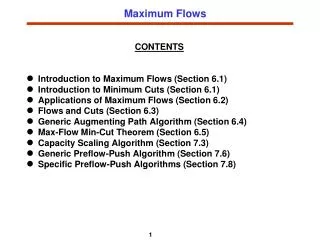
Maximum Flows. CONTENTS Introduction to Maximum Flows (Section 6.1) Introduction to Minimum Cuts (Section 6.1) Applications of Maximum Flows (Section 6.2) Flows and Cuts (Section 6.3) Generic Augmenting Path Algorithm (Section 6.4) Max-Flow Min-Cut Theorem (Section 6.5)

Maximum Flows
E N D
Presentation Transcript
Maximum Flows CONTENTS • Introduction to Maximum Flows (Section 6.1) • Introduction to Minimum Cuts (Section 6.1) • Applications of Maximum Flows (Section 6.2) • Flows and Cuts (Section 6.3) • Generic Augmenting Path Algorithm (Section 6.4) • Max-Flow Min-Cut Theorem (Section 6.5) • Capacity Scaling Algorithm (Section 7.3) • Generic Preflow-Push Algorithm (Section 7.6) • Specific Preflow-Push Algorithms (Section 7.8)
20 2 4 10 30 s t 15 40 1 6 35 20 25 3 5 35 Problem Definition Maximum Flow Problem: Given a directed network G with arc capacities given by uij’s, determine the maximum amount of flow that can be sent from a source node s to a sink node t. Decision Variables: Flow xij on arc (i, j), and the flow v entering the sink node.
A Linear Programming Problem The maximum flow problem can be formulated as the following linear programming problem: Maximize v subject to 0 xij uij for every arc (i, j) A
20 2 4 10 30 s t 15 40 1 6 35 25 25 3 5 Cost = -1, Capacity = 35 An Alternate Formulation The maximum flow problem can also be conceived of as the following minimum cost flow problem: Minimize -xts subject to lij xij uij for every arc (i, j) A
Assumptions • All arc capacities uij's are integer and U is the largest magnitudes of arc capacities. • The network is directed. • To satisfy this assumption, replace each undirected arc (i, j) with capacity uij by two directed arc (i, j) and (j, i) with capacity uij.
Minimum Cut Problem • A cut is a (minimal) set of arcs whose deletion from G disconnects the network (into two parts S and ). • An s-t cut is a cut that disconnects nodes s and t. • We denote an s-t cut as [S, ]. 20 2 4 15 10 30 s t 35 40 1 6 20 25 3 5 35
20 2 4 15 10 30 s t 35 40 1 6 20 25 3 5 35 Minimum Cut Problem (contd.) (S, ): Set of forward arcs in the cut [S, ] ( , S): Set of backward arcs in the cut [S, ] u[S, ] : Capacity of the cut [S, ] defined as
Assumptions 1. Network is directed. • How to satisfy this condition? 2. All arc capacities are nonnegative integers. Let U denote the largest arc capacity. 3. The network does not contain an uncapacitated (that is, infinite capacity) directed path from node s to node t. • How to identify such a possibility? 4. Whenever arc (i, j) is in A, (j, i) is also in A. • How to satisfy this condition? 5. The network does not contain parallel arcs. • How to eliminate this possibility?
Feasible Flow Problem In a sea-port network, merchandise is available at some sea-ports and desired at other ports. We know the supplies/ demands at various ports. Routes have capacities. Is it possible to satisfy the demands from the available supplies? Find a flow x satisfying the following constraints: 0 xij uij for every arc (i, j) A. The feasible flow problem is a feasibility version of the minimum cost flow problem. Notice: this requires that the sum of all b(i) be 0.
Feasible Flow Problem (contd.) Network G: Network G: • If the network G possesses a feasible flow, then the network G’ possesses a maximum flow that saturates all arcs emanating from the source node. • If the network G’ possesses a maximum flow saturating all arcs emanating from the source node, then the network G possesses a feasible flow. Supply nodes Demand nodes Supply nodes Demand nodes 5 1 4 5 b(5)<0 1 4 b(1)>0 b(1) -b(5) 3 3 t b(2) 2 s b(2)>0 2 7 7 -b(6) b(8) 8 6 9 b(8)>0 8 6 b(6)<0 9
Family nodes Table nodes uij =1 a(1) 1’ 1 -b(1) 2’ 2 a(2) -b(2) 3’ a(3) 3 -b(3) 4 a(4) Dining Problem Several families go out to dinner together. They would like to sit so that no two members of the same family are at the same table. How can they do it? Let the ith family have a(i) members and let the jth table have a seating capacity of b(j). The dining problem has a feasible solution if and only if the above network possesses a feasible solution.
Matrix Rounding Problem Given a p x q matrix of real numbers D = {dij} with row sums ai’s and column sums bj’s, round (up or down) the matrix elements dij’s, ai’s, and bj’s so that the matrix is consistent: • Row sums of the rounded elements equal the rounded row sums • Column sums of the rounded elements equal the rounded column sums • Determine such a consistent rounding if it exists.
[4,5] 1’ 1 [6,7] [13,14] [19,20] [9,10] [6,7] [16,17] t 2’ s 2 [8,9] [19,20] [4,5] [21,22] [3,4] [12,13] [1,2] 3’ 3 [7,8] Matrix Rounding Problem (contd.) Maximum Flow Formulation with Lower and Upper Bounds: There is a one-to-one correspondence between consistent roundings and feasible integer flows in the above network.
Flow Across an s-t Cut • The flow across a cut [S, ] is defined as the flow taking place on forward arcs minus the flow on backward arcs.
Properties of Flows and Cuts PROPERTY 1. The value of any flow is less than or equal to the capacity of any cut in the network. PROPERTY 2. Maximum flow value minimum cut capacity. PROPERTY 3. If the value of some flow x equals the capacity of some s-t cut [S, ], then x must be a maximum flow and [S, ] must be a minimum cut. Is maximum flow value = minimum cut capacity ? Yes! and we will prove it later.
(xij, uij) i j rij i j 2 3 5 1 1 2 4 1 1 2 3 Residual Network • Plays a central role in the development of maximum flow algorithms. • Defined with respect to a flow x. • Denotes how much flow can be sent on arcs with respect to a flow x. 2 [5,5] [3,4] [2,3] 4 1 [2,2] [0,1] 3
2 4 4 4 1 3 2 2 3 The Generic Augmenting Path Algorithm • Any directed path from node s to node t in the residual network is an augmenting path. • The generic augmenting path algorithm augments flow along augmenting paths until there are no augmenting paths.
The Generic Augmenting Path Algorithms (contd.) algorithm augmenting path; begin x := 0; while G(x) contain an augmenting path in G(x) do begin identify an augmenting path P; d := min {rij : (i, j) P}; augment x by d units along P and update G(x); end; end; • We can identify an augmenting path in O(m) time using a search algorithm. • The algorithm performs at most nU iterations. • The algorithm runs in O(nmU) time.
full 2 5 full 3 t 6 s 8 empty 7 9 1 empty Correctness of the Algorithm • Let the algorithm terminate with flow x*. Let S denote the set of nodes which are reachable in G(x) from the source node. Then • each forward arc in the cut [S, ] must have xij = uij • each backward arc in the cut [S, ] must have xij = 0 • The flow x* is a maximum flow and [S, ] is a minimum cut because the flow is equal to the capacity of the cut.
Some Theorems THEOREM 1 (Max-Flow Min-Cut Theorem). The maximum value of the flow from a source node s to a sink node t in a capacitated network equals the minimum capacity among all s-t cuts. THEOREM 2 (Augmenting Path Theorem). A flow x* is a maximum flow if and only if the residual network G(x*) contains no augmenting paths. THEOREM 3 (Integrality Theorem). If all arc capacities are integer, then the maximum flow problem has an integer maximum flow.
2 106 106 4 1 1 106 106 3 Drawbacks of Augmenting Path Algorithms • The algorithm may perform exponentially many iterations. • If arc capacities are irrational, then the algorithm might not terminate and the value it might converge to might be incorrect. • The algorithm does not make use of computations of the previous iterations.
Improved Augmenting Path Algorithms • SHORTEST AUGMENTING PATH ALGORITHM • Always augments flows along the shortest augmenting path in G(x), that is, containing the least number of arcs. • A breadth-first search of G(x) from node s will determine the shortest augmenting path in G(x). • The shortest augmenting path algorithm performs at most nm augmentations and can be implemented to run in O(n2m) time. • CAPACITY SCALING ALGORITHM • Proceeds by augmenting flows along paths of sufficiently large residual capacity. • The capacity scaling algorithm performs at most 2m(log U) augmentations and can be implemented in O(nm log U) time.
Capacity Scaling Algorithm • Is a specific implementation of the generic augmenting path algorithm. • Maintains a parameter D and performs a number of scaling phases. • In the D-scaling phase, it augments flow along an augmenting path with residual capacity at least D. • When there is no such path, it replaces D by D/2 and repeats the above process. • The algorithm terminates at the end of the D-scaling phase with D = 1. • The algorithm performs at most 2m augmentations in a scaling phase and O(m log U) overall.
40 2 4 10 30 s t 15 40 1 6 35 25 25 3 5 35 Example of Capacity Scaling Algorithm D-residual Network: A subgraph of G(x) containing only those arcs whose residual capacity is at least D.
Capacity Scaling Algorithm algorithm capacity-scaling; begin x: = 0; D : = 2log U; whileD 1 do begin while G(x, D) contains an augmenting path do begin {D-scaling phase} identify an augmenting path in G(x, D); l : = min{rij: (i, j) P}; augment l units along P and update G(x, D); end; {D-scaling phase} D : = D /2; end; end;
S rij < 2D 2 5 rij < 2D 3 t 6 s rij < 2D 8 7 9 1 rij < 2D Complexity Analysis of Capacity Scaling Algorithm • Consider the end of the 2D-scaling phase. • Let S denote the set of nodes which are reachable from the source node in G(x, 2D). • Each forward arc (i, j) in the cut [S, ] in G(x) has rij < 2D.
Complexity Analysis (contd.) • When the 2D-scaling phase ends, we can send at most 2mD units of additional flow. • In the D-scaling phase, each augmentation sends at least D units of flow. • The D-scaling phase will perform at most 2m augmentations. • The algorithm will perform at most O(m log U) augmentations. • The capacity scaling algorithm runs in O(m2 log U) time. • Capacity scaling algorithm can be implemented in O(nm log U) time.
Basic Features of Scaling Algorithms • Decompose the original problem into a sequence of approximate problems P1, P2, ..., PK, with each successive problem less approximate than the preceding problem. • The problem P1 is trivially solvable. • The problem PK is the original problem. • PK+1 is solved by reoptimizing the optimal solution of PK. • Works well when data are integral and reoptimization is much faster than solving the problem afresh.
11 1 1 12 1 1 13 1 1 14 1 1 15 1 1 16 21 10 1 1 1 1 17 2 1 5 1 18 1 1 3 3 6 1 1 19 8 7 9 1 20 Drawbacks of Augmenting Path Algorithms
Preflow-Push Algorithms • Substantially different than augmenting path algorithms. • Do not maintain mass balance constraints. • Are currently the fastest maximum flow algorithms (theoretically, as well as empirically). • Preflow-push algorithms maintain a preflow instead of a flow. • In a preflow x, inflow into any node is greater than or equal to its outflow:
Example of a Preflow • Excess of a node i is e(i) = • Nodes with positive excess are called active nodes 0 1 5 2 4 10 2 s t 0 2 1 6 5 20 20 3 5 20 2 5
Basic Idea • Maintain a preflow x. • Send excess flow from active node closer to the sink node. • Stop when no more flow can be sent to the sink node. 0 1 5 2 4 10 2 s t 0 2 1 6 5 20 20 3 5 20 2 5 • How to send flow closer to sink?
Distance Labels A set d(.) of distance labels associated with nodes satisfying • d(t) = 0; and • d(i) d(j) + 1 for all (i, j) in G(x) are called valid distance labels. 2 4 s t 1 6 3 5
Distance Labels (contd.) Valid Distance Labels: • There is no downward arc connecting nodes two or more layers across • d(t) = 0; and • d(i) d(j)+1 for all (i, j) in G(x) 3 1 2 2 3 2 4 5 1 1 6 0
1 2 3 4 5 6 d(3) 3 d(4) 2 d(5) 1 d(6)=0 d(1) 5 d(2) 4 Properties of Distance Labels PROPERTY 1. Any distance label d(i) is a lower bound on the length of the shortest path from node i to node t in G(x). Consider the following augmenting path: PROPERTY 2. If d(s) n, then G(x) has no augmenting path. Admissible Arc : An arc (i, j) in G(x) for which d(i) = d(j) + 1.
2 4 4 4 1 3 2 2 3 The Generic Algorithm • Establish an optimal preflow. • Select an active node i and push flow out of it using admissible arcs (i, j). • If node i has no admissible emanating from it, then increase its distance label (so that admissible arcs are created).
Algorithmic Description algorithmpreflow-push; begin pre-process; while the network contains an active node do begin select an active node i; push/relabel(i); end; end;
Algorithmic Description (contd.) procedurepre-process; begin x : = 0; compute the exact distance labels d(i); xsj : = usj for each arc (s, j) A(s); d(s) : = n; end; procedurepush/relabel(i); begin if the network contains an admissible arc then push : = min{e(i), rij} units of flow from node i to node j else replace d(i) by min{d(j) + 1 : (i, j) A(i) and rij > 0}; end; saturating push: : = rij non-saturating push: : = e(i)
Correctness and Complexity • Distance labels are valid throughout the algorithm. • The algorithm terminates when all the excess either reaches the sink node or comes back to the source node. Since d(s) = n, the flow is maximum. • Each relabel operation strictly increases a distance label. • For each node i N, d(i) = 2n. • Each distance label increases at most 2n times.
Correctness and Complexity (contd.) • The total number of relabel operations is at most 2n2. The time to perform relabel operations is O(nm). • Between two consecutive saturating pushes on an arc (i, j), both d(i) and d(j) must go up by at least 2 units. • The algorithm performs at most nm saturating pushes.
Correctness and Complexity (contd.) THEOREM. The algorithm performs O(n2m) nonsaturating pushes. PROOF. Let • The initial value of is at most 2n2. If the distance label of a node increases by units, then too increases by units. The total increase over the entire algorithm is 2n2. • Each saturating push increases by at most 2n units. The increase is at most 2n2m. • Each nonsaturating push decreases by at least one unit. Hence the number of nonsaturating pushes is at most 2n2 + 2n2 + 2n2m = O(n2m). THEOREM. The generic preflow-push algorithm runs in O(n2m) time.
Specific Implementations FIFO PREFLOW-PUSH ALGORITHM: • Examine active nodes in the FIFO order. Keep active nodes in a queue. • This algorithm runs in O(n3) time. HIGHEST-LABEL PREFLOW-PUSH ALGORITHM: • Always examine an active node with the highest distance label. • This algorithm also runs in O(n3) time. • Consider = max{d(i) : i is an active node}.