Download
1 / 49
490 likes | 505 Vues
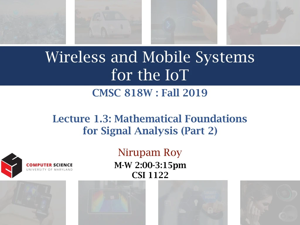
An overview of linear algebra and calculating the discrete Fourier transform for signal analysis in wireless and mobile systems.

E N D
Wireless and Mobile Systems for the IoT CMSC 818W : Fall 2019 • Lecture 1.3: Mathematical Foundations • for Signal Analysis (Part 2) Nirupam Roy M-W 2:00-3:15pm CSI 1122
An (incomplete) overview of Linear Algebra 2. Calculating Discrete Fourier Transform (DFT)
An (incomplete) overview of Linear Algebra 2. Calculating Discrete Fourier Transform (DFT)
Row view Solution, x=1, y=2
Column view What is the solution space or the set of all candidate solutions? Ans: All linear combinations of the columns of the matrix A(m x n)
Column space Solution space, spanned by the columns of the matrix A ( b vector should lie in this space )
What if the vectors are aligned? What is column rank of the matrix? A column is a linear combination of other columns i.e., the columns are not independent
Approximate solution Column space of the matrix A
Approximate solution Error e is orthogonal to the plane for optimal solution Projection of the vector b on the solution plane Two vectors a & b are orthogonal when their dot product (aTb) is zero.
Approximate solution Projection matrix
An (incomplete) overview of Linear Algebra 2. Calculating Discrete Fourier Transform (DFT)
Discrete Fourier Transform … Sample number X = [ ] x[0], x[1], x[2], x[3], x[4], … x[N-1] N-1 2 3 4 1 6 5 0
Discrete Fourier Transform … Sample number X = [ ] x[0], x[1], x[2], x[3], x[4], … x[N-1] N-1 2 3 4 1 6 5 0
Discrete Fourier Transform … Sample number N-1 2 3 4 1 6 5 0
Discrete Fourier Transform … Sample number = [ ] , … Freq f1 N-1 2 3 4 1 6 5 0
Discrete Fourier Transform … Sample number N-1 2 3 4 1 6 5 0
Discrete Fourier Transform … Sample number = [ ] , … Freq f2 N-1 2 3 4 1 6 5 0
Discrete Fourier Transform … Sample number What is the MINIMUM number of cycles observable in this model? N-1 2 3 4 1 6 5 0
Discrete Fourier Transform … Sample number N-1 2 3 4 1 6 5 0
Discrete Fourier Transform … Sample number = [ ] … , Freq f0 N-1 2 3 4 1 6 5 0
Discrete Fourier Transform … Sample number What is the MAXIMUM number of cycles observable in this model? N-1 2 3 4 1 6 5 0
Discrete Fourier Transform … Sample number What happens when the ball rotates exactly N times? N-1 2 3 4 1 6 5 0 We can uniquely observe up to (N-1) number of cycles.
Discrete Fourier Transform Freq f0 n=0 n=1 n=2 … … n=N-1
Discrete Fourier Transform Number of cycles … … Freq f0 Freq f1 Freqfm Freq fN-1 n=0 n=1 Sample number n=2 … … n=N-1
Discrete Fourier Transform Number of cycles … … Freq f0 Freq f1 Freqfm Freq fN-1 n=0 n=1 Sample number … … n=2 … … … … … n=N-1
Discrete Fourier Transform + + + Z1 Zm Z0 ZN-1 … … … … … …
Discrete Fourier Transform + + + Z1 Zm Z0 ZN-1 … … … … … …
Discrete Fourier Transform + + + Z1 Zm Z0 ZN-1 … … … … … … N-1 5 0 6 1 4 3 2 = … Sample number
Discrete Fourier Transform Frequency domain coefficients + + + Z1 Zm Z0 ZN-1 … … … … … … x[0] x[1] = X = Time domain samples x[2] … x[N-1]
Discrete Fourier Transform F … … fN-1 fm f1 f0 = DFT matrix,
Discrete Fourier Transform F … … fN-1 fm f1 f0 = DFT matrix, Z Z0 = Fourier coefficients, Z1 … Zm … ZN-1
Discrete Fourier Transform F … … fN-1 fm f1 f0 = DFT matrix, Z Z0 x[0] X = Time series, = Fourier coefficients, Z1 x[1] … x[2] Zm … … ZN-1 x[N-1]
Discrete Fourier Transform Z F X = X F-1 Z = * X F Z =
Discrete Fourier Transform Z F X = X F-1 Z = * X F Z = * f0 * f1 … * fm … * fN-1
Discrete Fourier Transform Z F X x[0] = x[1] X F-1 Z x[2] = … * X F Z x[N-1] = * Z0 f0 Z1 * … f1 Zm = … … * fm DFT IDFT ZN-1 … * fN-1
Discrete Fourier Transform z(m) = DFT: x(n) = IDFT:
Preserving energy in time and frequency domain Is IDFT( DFT(x) ) = x ?
Preserving energy in time and frequency domain Is IDFT( DFT(x) ) = x ? * * X ? N.X X X F F F F = = F … … fN-1 fm f1 f0 = DFT matrix,
Discrete Fourier Transform z(m) = DFT: x(n) = IDFT: