Download

1 / 99
1.04k likes | 1.37k Vues
Analysis of Algorithms. CSE 2320 – Algorithms and Data Structures Vassilis Athitsos University of Texas at Arlington. Analysis of Algorithms. Given an algorithm, some key questions to ask are: How efficient is this algorithm? Can we predict its running time on specific inputs?

E N D
Analysis of Algorithms CSE 2320 – Algorithms and Data Structures Vassilis Athitsos University of Texas at Arlington
Analysis of Algorithms • Given an algorithm, some key questions to ask are: • How efficient is this algorithm? • Can we predict its running time on specific inputs? • Should we use this algorithm or should we use an alternative? • Should we try to come up with a better algorithm? • Chapter 2 establishes some guidelines for answering these questions. • Using these guidelines, sometimes we can obtain easy answers. • At other times, getting the answers may be more difficult.
Empirical Analysis • This is an alternative to the more mathematically oriented methods we will consider. • Running two alternative algorithms on the same data and comparing the running times can be a useful tool. • 1 second vs. one minute is an easy-to-notice difference. • However, sometimes empirical analysis is not a good option. • For example, if it would take days or weeks to run the programs.
Data for Empirical Analysis • How do we choose the data that we use in the experiments?
Data for Empirical Analysis • How do we choose the data that we use in the experiments? • Actual data. • Pros: • Cons: • Random data. • Pros: • Cons: • Perverse data. • Pros: • Cons:
Data for Empirical Analysis • How do we choose the data that we use in the experiments? • Actual data. • Pros: give the most relevant and reliable estimates of performance. • Cons: may be hard to obtain. • Random data. • Pros: easy to obtain, make the estimate not data-specific. • Cons: may be too unrealistic. • Perverse data. • Pros: gives us worst case estimate, so we can obtain guarantees of performance. • Cons: the worst case estimate may be much worse than average performance.
Comparing Running Times • When comparing running times of two implementations, we must make sure the comparison is fair. • We are often much more careful optimizing "our" algorithm compared to the "competitor" algorithm. • Implementations using different programming languages may tell us more about the difference between the languages than the difference between implementations. • An easier case is when both implementations use mostly the same codebase, and differ in a few lines. • Example: the different implementations of Union-Find in Chapter 1.
Avoid Insufficient Analysis • Not performing analysis of algorithmic performance can be a problem. • Many (perhaps the majority) of programmers have no background in algorithms. • People with background in algorithmic analysis may be too lazy, or too pressured by deadlines, to use this background. • Unnecessarily slow software is a common consequence when skipping analysis.
Avoid Excessive Analysis • Worrying too much about algorithm performance can also be a problem. • Sometimes, slow is fast enough. • A user will not even notice an improvement from a millisecond to a microsecond. • The time spent optimizing the software should never exceed the total time saved by these optimizations. • E.g., do not spend 20 hours to reduce running time by 5 hours on a software that you will only run 3 times and then discard. • Ask yourself: what are the most important bottlenecks in my code, that I need to focus on? • Ask yourself: is this analysis worth it? What do I expect to gain?
Mathematical Analysis of Algorithms • Some times it may be hard to mathematically predict how fast an algorithm will run. • However, we will study a relatively small set of techniques that applies on a relatively broad range of algorithms. • First technique: find key operationsand key quantities. • Identify the important operations in the program that constitute the bottleneck in the computations. • This way, we can focus on estimating the number of times these operations are performed, vs. trying to estimate the number of CPU instructions and/or nanoseconds the program will take. • Identify a few key quantities that measure the size of the data that determine the running time.
Finding Key Operations • We said it is a good idea to identify the important operations in the code, that constitute the bottleneck in the computations. • How can we do that?
Finding Key Operations • We said it is a good idea to identify the important operations in the code,that constitute the bottleneck in the computations. • How can we do that? • One approach is to just think about it. • Another approach is to use software profilers, which show how much time is spent on each line of code.
Finding Key Operations • What were the key operations for Union Find? • ??? • What were the key operations for Binary Search? • ??? • What were the key operations for Selection Sort? • ???
Finding Key Operations • What were the key operations for Union Find? • Checking and changing ids in Find. • Checking and changing ids in Union. • What were the key operations for Binary Search? • Comparisons between numbers. • What were the key operations for Selection Sort? • Comparisons between numbers. • In all three cases, the running time was proportional to the total number of those key operations.
Finding Key Quantities • We said that it is a good idea to identify a few key quantities that measure the size of the data and that are the most important in determining the running time. • What were the key quantities for Union-Find? • ??? • What were the key quantities for Binary Search? • ??? • What were the key quantities for Selection Sort? • ???
Finding Key Quantities • We said that it is a good idea to identify a few key quantities that measure the size of the data and that are the most important in determining the running time. • What were the key quantities for Union-Find? • Number of nodes, number of edges. • What were the key quantities for Binary Search? • Size of the array. • What were the key quantities for Selection Sort? • Size of the array.
Finding Key Quantities • These key quantities are different for each set of data that the algorithm runs on. • Focusing on these quantities greatly simplifies the analysis. • For example, there is a huge number of integer arrays of size 1,000,000, that could be passed as inputs to Binary Search or to Selection Sort. • However, to analyze the running time, we do not need to worry about the contents of these arrays (which are too diverse), but just about the size, which is expressed as a single number.
Describing Running Time • Rule: most algorithms have a primary parameter N, that measures the size of the data and that affects the running time most significantly. • Example: for binary search, Nis ??? • Example: for selection sort, N is ??? • Example: for Union-Find, N is ???
Describing Running Time • Rule: most algorithms have a primary parameter N, that measures the size of the data and that affects the running time most significantly. • Example: for binary search, Nis the size of the array. • Example: for selection sort, N is the size of the array. • Example: for Union-Find, N is ??? • Union-Find is one of many exceptions. • Two key parameters, number of nodes, and number of edges, must be considered to determine the running time.
Describing Running Time • Rule: most algorithms have a primary parameter N, that affects the running time most significantly. • When we analyze an algorithm, our goal is to find a function f(N), such that the running time of the algorithm is proportionalto f(N). • Why proportional and not equal?
Describing Running Time • Rule: most algorithms have a primary parameter N, that affects the running time most significantly. • When we analyze an algorithm, our goal is to find a function f(N), such that the running time of the algorithm is proportionalto f(N). • Why proportional and not equal? • Because the actual running time is not a defining characteristic of an algorithm. • Running time depends on programming language, actual implementation, compiler used, machine executing the code, …
Describing Running Time • Rule: most algorithms have a primary parameter N, that affects the running time most significantly. • When we analyze an algorithm, our goal is to find a function f(N), such that the running time of the algorithm is proportionalto f(N). • We will now take a look at the most common functions that are used to describe running time.
The Constant Function: f(N) = 1 • f(N) = 1. What does it mean to say that the running time of an algorithm is described by 1?
The Constant Function: f(N) = 1 • f(N) = 1. What does it mean to say that the running time of an algorithm is described by 1? • It means that the running time of the algorithm is proportional to 1, which means…
The Constant Function: f(N) = 1 • f(N) = 1: What does it mean to say that the running time of an algorithm is described by 1? • It means that the running time of the algorithm is proportional to 1, which means… • that the running time is constant, or at least bounded by a constant. • This happens when all instructions of the program are executed only once, or at least no more than a certain fixed number of times. • If f(N) = 1, we say that the algorithm takes constant time. This is the best case we can ever hope for.
The Constant Function: f(N) = 1 • What algorithm (or part of an algorithm) have we seen whose running time is constant?
The Constant Function: f(N) = 1 • What algorithm (or part of an algorithm) have we seen whose running time is constant? • The find operation in the quick-find version of Union-Find.
Logarithmic Time: f(N) = log N • f(N) = log N: the running time is proportional to the logarithm of N. • How good or bad is that?
Logarithmic Time: f(N) = log N • f(N) = log N: the running time is proportional to the logarithm of N. • How good or bad is that? • log 1000 ~= ???. • The logarithm of one million is about ???. • The logarithm of one billion is about ???. • The logarithm of one trillion is about ???.
Logarithmic Time: f(N) = log N • f(N) = log N: the running time is proportional to the logarithm of N. • How good or bad is that? • log 1000 ~= 10. • The logarithm of one million is about 20. • The logarithm of one billion is about 30. • The logarithm of one trillion is about 40. • Function log N grows very slowly: • This means that the running time when N = one trillion is only four times the running time when N = 1000. This is really good scaling behavior.
Logarithmic Time: f(N) = log N • If f(N) = log N, we say that the algorithm takes logarithmic time. • What algorithm (or part of an algorithm) have we seen whose running time is proportional to log N?
Logarithmic Time: f(N) = log N • If f(N) = log N, we say that the algorithm takes logarithmic time. • What algorithm (or part of an algorithm) have we seen whose running time is proportional to log N? • Binary Search. • The Find function on the weighted-cost quick-union version of Union-Find.
Logarithmic Time: f(N) = log N • Logarithmic time commonly occurs when solving a big problem is solved in a sequence of steps, where: • Each step reduces the size of the problem by some constant factor. • Each step requires no more than a constant number of operations. • Binary search is an example: • Each step reduces the size of the problem by a factor of 2. • Each step requires only one comparison, and a few variable updates.
Linear Time: f(N) = N • f(N) = N: the running time is proportional to N. • This happens when we need to do some fixed amount of processing on each input element. • What algorithms (or parts of algorithms) are examples?
Linear Time: f(N) = N • f(N) = N: the running time is proportional to N. • This happens when we need to do some fixed amount of processing on each input element. • What algorithms (or parts of algorithms) are examples? • The Union function in the quick-find version of Union-Find. • Sequential search for finding the min or max value in an array. • Sequential search for determining whether a value appears somewhere in an array. • Is this ever useful? Can't we always just do binary search?
Linear Time: f(N) = N • f(N) = N: the running time is proportional to N. • This happens when we need to do some fixed amount of processing on each input element. • What algorithms (or parts of algorithms) are examples? • The Union function in the quick-find version of Union-Find. • Sequential search for finding the min or max value in an array. • Sequential search for determining whether a value appears somewhere in an array. • Is this ever useful? Can't we always just do binary search? • If the array is not already sorted, binary search does not work.
N log N Time • f(N) = N log N: the running time is proportional to N log N. • This running time is commonly encountered, especially in algorithms working as follows: • Break problem into smaller subproblems. • Solve subproblems independently. • Combine the solutions of the subproblems. • Many sorting algorithms have this complexity. • Comparing linear to N log N time. • N = 1 million, N log N is about ??? • N = 1 billion, N log N is about ??? • N = 1 trillion, N log N is about ???
N log N Time • Comparing linear to N log N time. • N = 1 million, N log N is about 20 million. • N = 1 billion, N log N is about 30 billion. • N = 1 trillion, N log N is about 40 trillion. • N log N is worse than linear time, but not by much.
Quadratic Time • f(N) = N2: the running time is proportional to the square of N. • In this case, we say that the running time is quadratic to N. • Any example where we have seen quadratic time?
Quadratic Time • f(N) = N2: the running time is proportional to the square of N. • In this case, we say that the running time is quadratic to N. • Any example where we have seen quadratic time? • Selection Sort.
Quadratic Time • Comparing linear, N log N, and quadratictime. • Quadratic time algorithms become impractical (too slow) much faster than linear and N log N time algorithms. • Of course, what we consider "impractical" depends on the application. • Some applications are more tolerant of longer running times.
Cubic Time • f(N) = N3: the running time is proportional to the cube of N. • In this case, we say that the running time is cubic to N.
Cubic Time • Example of a problem whose solution has cubic running time: the assignment problem. • We have two sets A and B. Each set contains N items. • We have a cost function C(a, b), assigning a cost to matching an item a of A with an item b of B. • Find the optimal one-to-one correspondence (i.e., a way to match each element of A with one element of B and vice versa), so that the sum of the costs is minimized.
Cubic Time • Wikipedia example of the assignment problem: • We have three workers, Jim, Steve, and Alan. • We have three jobs that need to be done. • There is a different cost associated with each worker doing each job. • What is the optimal job assignment? • Cubic running time means that it is too slow to solve this problem for, let's say, N = 1 million.
Exponential Time • f(N) = 2N: this is what we call exponential running time. • Such algorithms are usually too slow unless N is small. • Even for N = 100, 2N is too large and the algorithm will not terminate in our lifetime, or in the lifetime of the Universe. • Exponential time arises when we try all possible combinations of solutions. • Example: travelling salesman problem: find an itinerary that goes through each of N cities, visits no city twice, and minimizes the total cost of the tickets. • Quantum computers (if they ever arrive) may solve some of these problems with manageable running time.
Some Useful Constants and Functions These tables are for reference. We may use such symbols and functions as we discuss specific algorithms.
Motivation for Big-Oh Notation • Given an algorithm, we want to find a function that describes the running time of the algorithm. • Key question: how much data can this algorithm handle in a reasonable time? • There are some details that we would actually NOT want this function to include, because they can make a function unnecessarily complicated. • Constants. • Behavior fluctuations on small data. • The Big-Oh notation, which we will see in a few slides, achieves that, and greatly simplifies algorithmic analysis.
Why Constants Are Not Important • Does it matter if the running time is f(N) or 5*f(N)?
Why Constants Are Not Important • Does it matter if the running time is f(N) or 5*f(N)? • For the purposes of algorithmic analysis, it typically does NOT matter. • Constant factors are NOT an inherent property of the algorithm. They depend on parameters that are independent of the algorithm, such as: • Choice of programming language. • Quality of the code. • Choice of compiler. • Machine capabilities (CPU speed, memory size, …)
Why Asymptotic Behavior Matters • Asymptotic behavior: The behavior of a function as the input approaches infinity. h*f(N) c*f(N) N: Size of data g(N) f(N) Running Time for input of size N