Download
1 / 59
630 likes | 1.04k Vues
Validation Olivier Talagrand WMO Workshop on 4D-Var and Ensemble Kalman Filter Intercomparisons Buenos Aires, Argentina 13 November 2008.

E N D
Validation Olivier TalagrandWMO Workshop on 4D-Var and Ensemble Kalman Filter IntercomparisonsBuenos Aires, Argentina13 November 2008
Purpose of assimilation : reconstruct as accurately as possible the state of the atmospheric or oceanic flow, using all available appropriate information. The latter essentially consists of • The observations proper, which vary in nature, resolution and accuracy, and are distributed more or less regularly in space and time. • The physical laws governing the evolution of the flow, available in practice in the form of a discretized, and necessarily approximate, numerical model. • ‘Asymptotic’ properties of the flow, such as, e. g., geostrophic balance of middle latitudes. Although they basically are necessary consequences of the physical laws which govern the flow, these properties can usefully be explicitly introduced in the assimilation process.
Validation must therefore aim primarily at determining, as far as possible, the accuracy with which assimilation reconstructs the state of the flow. In particular, if one wants to compare two different assimilation procedures, the ultimate test lies in the comparison of the accuracies with which those two procedures reconstruct the flow. Now, the state of the flow is not perfectly known, and the output of an assimilation process is precisely meant to be the best possible estimate of that state. So there is a circular argument there.
But there is another aspect to evaluation of an assimilation process. Does the process make the best possible use of the available information ? This is totally distinct from the accuracy with which the process reconstructs the state of the flow. We will distinguish numerical accuracy from optimality (the property that the process makes the best possible use of the available information).
Objective validation of assimilation can only be statistical, and must be made against observations (or data) that are unbiased, and are affected by errors that are statistically independent of the errors affecting the data used in the assimilation. Amplitude of forecast error, if estimated against observations that are really independent of observations used in assimilation, is an objective measure of accuracy of assimilation. But neither the unbiasedness nor the ‘independence’ of the verifying observations can be objectively verified, at least within the world of data and assimilation. External knowledge must be used.
Best Linear Unbiased Estimate State vectorx, belonging to state spaceS (dimS = n), to be estimated. Available data in the form of • A ‘background’ estimate, belonging to state space, with dimension n xb = x+ b • An additional set of data (e. g. observations), belonging to observation space, with dimension p y = Hx + H is known linear observation operator.
Best Linear Unbiased Estimate (continuation 2) Assume E(b) = 0, E() = 0 Set dy - Hxb (innovation vector) xa = xb- E(bdT) [E(ddT)]-1(y - Hxb) Pa =E(bbT) - E(bdT) [E(ddT)]-1 E(dbT) Assume E(bT) = 0 (not restrictive). Set E(bbT) = Pb (also often denoted B), E(T) = R xa = xb+PbHT[HPbHT + R]-1(y - Hxb) Pa = Pb- PbHT[HPbHT + R]-1HPb xa is the Best Linear Unbiased Estimate (BLUE) of xfrom xb and y. If probability distributions are globally gaussian, BLUE achieves bayesian estimation, in the sense that P(x| xb, y) = N [xa, Pa]. Determination of the BLUE requires (at least apparently) the a priori specification of the expectation and covariance matrix, i. e. the statistical moments of orders 1 and 2 of the errors. The expectation is required for unbiasing the data in the first place.
Questions • Is itpossible to objectively evaluatethe accuracy of an assimilation system? • Is itpossible to objectively evaluatethe first- and second-order statistical moments of the data errors, whose specification is required for determining the BLUE ? • Is itpossible to objectively determine whether an assimilation system is optimal(i. e., in the case of the BLUE, whether it uses the correct error statistics) ? • More generally, how to make the best of an assimilation system?
xb = x+ b y = Hx + The only combination of the data that is a function of only the error is the innovation vector d = y - Hxb = - Hb (if H weakly nonlinear, d = - H’b ,where H’is local jacobian) Innovation is the only objective source of information on errors. Now innovation is a combination of background and observation errors, while determination of the BLUE requires explicit knowledge of the statistics of both observation and background errors. xa = xb+ PbHT[HPbHT + R]-1(y - Hxb) Innovation alone will never be sufficient to determine the required statistics.
With hypotheses made above E(d) = 0 ; E(ddT) = HPbHT + R Possible to checkstatistical consistency between a priori assumed and a posteriori observed statistics of innovation. Consistency, which will be considered now, is a different quality than either accuracy or optimality. Consider assimilation scheme of the form xa = xb+ K(y - Hxb) (1) with any (i. e. not necessarily optimal) gain matrix K. (1) if data are perfect, then so is the estimate xa.
Take more general approach. Dataassumed to consist of a vector z, belonging to data space D (dimD = m), in the form z = x + whereis a known (mxn)-matrix, and an unknown ‘error’ For instance which corresponds to
Look for estimated state vector xaof the form xa = + Az subject to • invariance in change of origin in state space A= Im • quadratic estimation error E[(xai - xi)2] minimum for any component xi.
Solution xa = (T S-1)-1TS-1 [z ] PaE[(xa - x) (xa - x)T] = (T S-1)-1 where ) , S E(’’T) , ’ Requires (at least apparently) a priori explicit knowledge of ) and E(’’T) Unambiguously defined iff rank= n. Determinacy condition. Requires m ≥ n. We shall set m = n + p. Invariant in any invertible linear change of coordinates, either in data or state space. In case is gaussian, = N [, S],BLUE achieves bayesian estimation in the sense that P(xz) = N [xa, Pa]
If determinacy condition is verified, it is always possible to decompose data vector zinto xb = x+ b y = Hx + with E(b) = 0 ; E() = 0 ; E(bT) = 0 xais the same estimate (BLUE) as before, viz., xa = xb+PaHTR-1(y - Hxb) [Pa]-1 = [Pb]-1+ HTR-1H xa = xb+PbHT[HPbHT + R]-1(y - Hxb) Pa = Pb- PbHT[HPbHT + R]-1HPb
Data have been put in the format xb = x+ b d= y - Hxb = - Hb through linear invertible transformation Assume that, through further linear invertible transformation, I put data in format u = Cx+ v = where C is invertible, and and are functions of the original error only u = Bxb + Dd v = Exb + Fd with necessarily EC = 0 E = 0 Then v = Fd, with F invertible Conclusion. Innovation is much more than observation-minus-background difference, it is what one obtains by eliminating the unknowns from the data, independently of how elimination is performed.
Conclusion. Innovation is much more than observation-minus-background difference, it is what one obtains by eliminating the unknowns from the data, independently of how elimination is performed. Extends to nonlinear situations.
One particular form of elimination Linear analysis (whether optimal or not) xa = x+ a Data-minus-analysis difference z - xa = -a + Data-minus-analysis difference is in one-to-one correspondance with the innovation. It is exactly equivalent to compute statistics on either the innovation d or on the DmA difference .
For perfectly consistent system (i. e., system that uses the exact error statistics): E(d) = 0(E() = 0) Any systematic bias in either the innovation vector or the DmA difference is the signature of an inappropriately taken into account bias in either the background or the observation (or both). E[(xb-xa)(xb-xa)T] = Pb - Pa E[(y- Hxa)(y- Hxa)T] = R- HPaHT A perfectly consistent analysis statistically fits the data to within their own accuracy. If new data are added to (removed from) an optimal analysis system, DmA difference must increase (decrease).
Also (Desroziers et al., 2006, QJRMS) E[H(xa-xb)(y-Hxb)T] = E[H(xa-xb)dT] = HPbHT E[(y-Hxa)(y-Hxb)T] = E[(y-Hxa)dT] = R
Assume inconsistency has been found between a priori assumed and a posteriori observed statistics of innovation or DmA difference. - What can be done ? or, equivalently - Which bounds does the knowledge of the statistics of innovation put on the error statistics whose knowledge is required by the BLUE ?
Come back to global data format z = x + whereis a known (mxn)-matrix, and an unknown ‘error’
Variational form. xaminimizes following scalar objective function, defined on state space S J() (1/2) [- (z-)]TS-1 [- (z-)] (Mahalanobis S-metric)
J() (1/2) [- (z-)]TS-1 [- (z-)] z- xa (S)
Minimizing J() amounts to • unbias z • project orthogonally onto space (S) according to Mahalanobis S-metric • take inverse through (inverse unambiguously defined through determinacy condition)
Many assimilation methods - Optimal Interpolation - 3DVar, either primal or dual - Kalman Filter, either in its simple or Extended form - Kalman Smoother - 4DVar, either in its strong- or weak-constraint form, or in its primal or dual form areparticular cases of that general scheme. Only exceptions (so far) - Ensemble Kalman Filter (which is linear however in its ‘updating’ phase) - Particle Filters
Decompose data space D into image space (S)(index 1) and its S-orthogonal space (S) (index 2) 1 invertible Assume Then xa = 1 -1[z1 1]
xa = 1 -1[z1 1] The probability distribution of the error xa - x = 1 -1[1 1] depends on the probability distribution of 1. On the other hand, the probability distribution of = (z-) - xa = depends only on the probability distribution of 2.
DmA difference, i. e. (z-) - xa, is in effect ‘rejected’ by the assimilation. Its expectation and covariance are irrelevant for the assimilation. Consequence. Any assimilation scheme (i. e., a priori subtracted bias and gain matrix K) is compatible with any observed statistics of either DmA or innovation. Not only is not consistency between a priori assumed and a posteriori observed statistics of innovation (or DmA) sufficient for optimality of an assimilation scheme, it is not even necessary.
Example z1 = x + 1 z2 = x + 2 Errors 1and2 assumed to be centred (E(1) = E(2) = 0), to have same variance s and to be mutually uncorrelated. Then xa = (1/2) (z1 + z2) with expected quadratic estimation error E[(xa-x)2] = s/2 Innovation is difference z1 - z2. With above hypotheses, one expects to observe E(z1 - z2) = 0 ; E[(z1 - z2)2] = 2s Assume one observes E(z1 - z2) = b ; E[(z1 - z2)2] = b2+ 2g Inconsistency if b≠0 and/or ≠s
Inconsistency can always be resolved by assuming that E(1) = -E(2) = -b/2 E(’12) = E(’22) = (s+)/2 E(’1’2) = (s-)/2 This alters neither the BLUExa, nor the corresponding quadratic estimation error E[(xa-x)2].
Explanation. It is not necessary to know explicitly the complete expectation and covariance matrix S in order to perform the assimilation. It is necessary to know the projection of and S onto the subspace (S). As for the subspace that is S-orthogonal to (S), it suffices to know what it is, but it is not necessary to know the projection of and S onto it. A number of degrees of freedom are therefore useless for the assimilation. The parameters determined by the statistics of d are equal in number to those useless degrees of freedom, to which any inconsistency between a priori and a posteriori statistics of the innovation can always mathematically be attributed. Howeverit may be that resolving the inconsistency in that way requires conditions that are (independently) known to be very unlikely, if not simply impossible. For instance, in the above example, consistency when ≠s requires the errors 1 and 2 to be mutually correlated, which may be known to be very unlikely.
J() (1/2) [- (z-)]TS-1 [- (z-)] z- xa (S)
That result, which is purely mathematical, means that the specification of the error statistics required by the assimilation must always be based, in the last resort, on external hypotheses, i. e. on hypotheses that cannot be validated on the basis of the innovation alone. Now, such knowledge always exists in practice. Problem. Identify hypotheses • That will not be questioned (errors on observations performed a long distance apart by radiosondes made by different manufacturers are uncorrelated) • That sound reasonable, but may be questioned (observation and background errors are uncorrelated) • That are undoubtedly questionable (model errors are negligible) Ideally,define a minimum set of hypotheses such that all remaining undetermined error statistics can be objectively determined from observed statistics of innovation.
Objective function J() (1/2) [- z]TS-1 [- z] JminJ(xa) = (1/2) [xa- z]TS-1 [xa- z] = (1/2) dT[E(ddT)]-1d E(Jmin) = p/2 (p = dimy = dimd) Ifpis large, a few realizations are sufficient for determiningE(Jmin) Often called2criterion. Remark. If in addition errors are gaussian Var(Jmin) = p/2
Results for ECMWF (January 2003, n = 8 106) - Operations (p = 1.4 106, has significantly increased since then) 2Jmin /p= 0.40 - 0.45 Innovation is significantly smaller thanimplied by Pb and R(a residual bias in d would make Jmin too large). - Assimilation without satellite observations (p = 2 - 3 105) 2Jmin /p= 1. - 1.05 Similar results obtained at other NWP centres (C. Fischer, W. Sadiki with Aladin model, T. Payne at Meteorological Office, UK). Probable explanation: error variance of satellite observations overestimated in order to compensate for ignored spatial correlation.
Informative content Objective function J() k Jk() where Jk() (1/2) (Hk- yk)TSk-1(Hk- yk) withdimyk=mk Accuracy of analysis Pa = (T S-1)-1 [Pa]-1k HkTSk-1 Hk (1/n) k tr(Pa HkTSk-1 Hk) (1/n) k tr(Sk–1/2 Hk Pa HkTSk–1/2)
Informative content (continuation 1) (1/n) k tr(Sk–1/2 Hk Pa HkTSk–1/2) = 1 I(yk) (1/n) tr(Sk–1/2 Hk Pa HkTSk–1/2) is a measure of the relative contribution of subset of data yk to overall accuracy of assimilation. Invariant in linear change of coordinates in data space valid for any subset of data. In particular I(xb) = (1/n) tr[Pa (Pb)-1] = 1 - (1/n) tr(KH) I(y) = (1/n) tr(KH) Rodgers, 2000, calls those quantities Degrees of Freedom for Signal,or for Noise,depending on whether considered subset belongs to ‘observations’ or ‘background’. See also papers by C. Cardinali, M. Fisher and others.
Informative content of subsets of observations (Arpège Assimilation System, Météo-France) Chapnik et al., 2006, QJRMS, 132, 543-565
Informative content per individual (scalar) observation (courtesy B. Chapnik)
Objective function J() k Jk() where Jk() (1/2) (Hk- yk)TSk-1(Hk- yk) with dimyk=mk For a perfectly consistent system E[Jk(xa)] (1/2) [mk - tr(Sk–1/2 Hk Pa HkTSk–1/2)] (in particular, E(Jmin) = p/2) For same vector dimension mk, more informative data subsets lead at the minimum to smaller terms in the objective function.
Equality E[Jk(xa)] (1/2) [mk - tr(Sk–1/2 Hk Pa HkTSk–1/2)] (1) can be objectively checked. Chapnik et al. (2004, 2005). Multiply each observation error covariance matrix Sk by a coefficient k such that (1) is verified simultaneously for all observation types. System of equations fot the k‘s solved iteratively.
Chapnik et al., 2006, QJRMS, 132, 543-565
Informative content (continuation 2) I(yk) (1/n) tr(Sk–1/2 Hk Pa HkTSk–1/2) Two subsets of data z1 and z2 If errors affecting z1 and z2 are uncorrelated, then I(z1 z2) = I(z1) + I(z2) If errors are correlated I(z1 z2) ≠ I(z1) + I(z2)
Informative content (continuation 3) Example 1 z1 = x + 1 z2 = x + 2 Errors 1and2 assumed to centred, to have same variance and correlation coefficient c. I(z1) =I(z2) = (1/2) (1 + c) More generally, two sets of data z1 and z2 can be said to be positively correlated if I(z1 z2) < I(z1) + I(z2), andnegatively correlated if I(z1 z2) > I(z1) + I(z2).
Informative content (continuation 4) Example 2 State vector x evolving in time according to x2 = x1 Observations are performed at times 1 and 2. Observation errors are assumed centred, uncorrelated and with same variance 2. Information contents are then in ratio (1, 2). For an unstablesystem (>1), laterobservation contains more information(and the opposite for a stable system). If model error is present, viz. x2 = x1 + uncorrelated with observation errors, E(2) = 2, then informative contents in observation at time 1, observation at time 2 and in model are in the proportion (1+, 2+, 1+2).
Informative content (continuation 5) Subset u1of analyzed fields, dimu1 = n1. Define relative contribution of subset yk of data to accuracy of u1? u2: component of xorthogonal to u1with respect to Mahalanobis norm associated with Pa (analysis errors on u1 and u2 are uncorrelated). x= (u1T,u2T)T. In basis (u1, u2)
Informative content (continuation 6) Observation operator Hk decomposes into Hk = (Hk1, Hk2) and expression of estimation error covariance matrix into [Pa1]-1k Hk1TSk-1 Hk1 [Pa2]-1k Hk2TSk-1 Hk2 Same development as before shows that the quantity (1/n1) tr(Sk–1/2 Hk1 Pa1Hk1TSk–1/2) is a measure of the relative contribution of subset yk of data to analysis of subset u1 of state vector. But can it be computed in practice for large dimension systems (requires the explicit decomposition x= (u1T,u2T)T) ?
If we accept to systematically describe uncertainty by probability distributions (see, e. g., Jaynes, 2007), then assimilation can be stated as a problem in bayesian estimation Determine the conditional probability distribution for the state of the system, knowing everything that is known (unambiguously defined if a prior probability distribution is defined; see Tarantola, 2005).
Questions are now • Is itpossible to objectively evaluatewhether the system achieves bayesian estimation ? • Is itpossible to objectively determinethe probability distributions which describe the uncertainty on the data?
‘Bayesianity’ of estimation. Conditional probability distribution that it sought is meant to describe our uncertainty on the state of the system. As such, it depends on elements (such as our present state of knowledge of the physical laws that govern the system) that cannot influence whatever we can observe.