Download
1 / 146
1.53k likes | 1.88k Vues
Formation Flying in Earth, Libration, and Distant Retrograde Orbits David Folta NASA - Goddard Space Flight Center Advanced Topics in Astrodynamics Barcelona, Spain July 5-10, 2004. Agenda. I. Formation flying – current and future II. LEO Formations

E N D
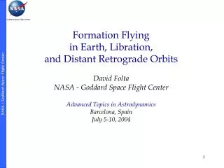
Formation Flying in Earth, Libration, and Distant Retrograde Orbits David Folta NASA - Goddard Space Flight Center Advanced Topics in Astrodynamics Barcelona, Spain July 5-10, 2004
Agenda • I. Formation flying – current and future • II. LEO Formations • Background on perturbation theory / accelerations • - Two body motion • - Perturbations and accelerations • LEO formation flying • - Rotating frames • - Review of CW equations, Shuttle • - Lambert problems, • - The EO-1 formation flying mission • III. Control strategies for formation flight in the vicinity of the libration points • Libration missions • Natural and controlled libration orbit formations • - Natural motion • - Forced motion • IV. Distant Retrograde Orbit Formations • V. References • All references are textbooks and published papers • Reference(s) used listed on each slide, lower left, as ref#
NASA Themes and Libration Orbits NASA Enterprises of Space Sciences (SSE) and Earth Sciences (ESE) are a combination of several programs and themes SSE ESE SEU Origins SEC • Recent SEC missions include ACE, SOHO, and the L1/L2 WIND mission. The Living With a Star (LWS) portion of SEC may require libration orbits at the L1 and L3 Sun-Earth libration points. • Structure and Evolution of the Universe (SEU) currently has MAP and the future Micro Arc-second X-ray Imaging Mission (MAXIM) and Constellation-X missions. • Space Sciences’ Origins libration missions are the James Webb Space Telescope (JWST) and The Terrestrial Planet Finder (TPF). • The Triana mission is the lone ESE mission not orbiting the Earth. • A major challenge is formation flying components of Constellation-X, MAXIM, TPF, and Stellar Imager. Ref #1
Earth Science Low Earth Orbit Formations • The ‘a.m.’ train • ~ 705km, 980 inclination, • 10:30 .pm. Descending node sun-sync • -Terra (99): Earth Observatory • - Landsat-7(99): Advanced land imager • -SAC-C(00): Argentina s/c • -EO-1(00) : Hyperspectral inst. • The ‘p.m.’ train • ~ 705km, 980 inclination, • 1:30 .pm. Ascending node sun-sync • - Aqua (02) • - Aura (04) • - Calipso (05) • CloudSat (05) • Parasol (04) • - OCO (tbd) Ref # 1, 2
FKSI (Fourier Kelvin Stellar Interferometer): near IR interferometer JWST (James Webb Space Telescope): deployable, ~6.6 m, L2 Constellation – X: formation flying in librations orbit SAFIR (Single Aperture Far IR): 10 m deployable at L2, Deep space robotic or human-assisted servicing Membrane telescopes Very Large Space Telescope (UV-OIR): 10 m deployable or assembled in LEO, GEO or libration orbit MAXIM: Multiple X ray s/c Stellar Imager: multiple s/c form a fizeau interferometer TPF (Terrestrial Planet Finder): Interferometer at L2 30 m single dish telescopes SPECS (Submillimeter Probe of the Evolution of Cosmic Structure): Interferometer 1 km at L2 Space Science Launches Possible Libration Orbit missions Ref #1
Future Mission Challenges Considering science and operations • Orbit Challenges • Biased orbits when using large sun shades • Shadow restrictions • Very small amplitudes • Reorientation and Lissajous classes • Rendezvous and formation flying • Low thrust transfers • Quasi-stationary orbits • Earth-moon libration orbits • Equilateral libration orbits: L4 & L5 • Science Challenges • Interferometers • Environment • Data Rates • Limited Maneuvers • Operational Challenges • Servicing of resources in libration orbits • Minimal fuel • Constrained communications • Limited DV directions • Solar sail applications • Continuous control to reference trajectories • Tethered missions • Human exploration
Background on perturbation • theory / accelerations • Two Body Motion • Atmospheric Drag • Potential Models Forces • Solar Radiation Pressure
Two – Body Motion • Newton’s law of gravity of force is inversely proportional to distance • Vector direction from r2 to r1 and r1 to r2 • Subtract one from other and define vector r, and gravitational constants Fundamental Equation of Motion Ref # 3-7
Equation Of Motion Propagated. External Accelerations Caused By Perturbations FORCES ONPROPAGATED ORBIT + accelerations a = anonspherical+adrag+a3body+asrp+atides+aother Ref #3-7
Changes in Keplerian motion due to perturbations in terms of the applied force. These are a set of differential equations in orbital elements that provide analytic solutions to problems involving perturbations from Keplerian orbits. For a given disturbing function, R, they are given by Gaussian Lagrange Planetary Equations Ref # 3-7
Geopotential • Spherical Harmonics break down into three types of terms • Zonal – symmetrical about the polar axis • Sectorial – longitude variations • Tesseral – combinations of the two to model specific regions • J2 accounts for most of non-spherical mass • Shading in figures indicates additional mass Ref # 3-7
The coordinates of P are now expressed in spherical coordinates , where is the geocentric latitude and is the longitude. R is the equatorial radius of the primary body and is the Legendre’s Associated Functions of degree and order m. The coefficients and are referred to as spherical harmonic coefficients. If m = 0 the coefficients are referred to as zonal harmonics. If they are referred to as tesseral harmonics, and if , they are called sectoral harmonics. Simplified J2 acceleration model for analysis with acceleration in inertial coordinates -3J2mRe2 ri 5rk2 r2 1- ai = 2r5 df + df + df dx + dy + dz a = f = i j k D -3J2mRe2 rj 5rk2 r2 1- aj = 2r5 -3J2mRe2 rj 5rk2 r2 3- ak = 2r5 Potential Accelerations Ref # 3-7
Atmospheric Drag Force On The Spacecraft Is A Result Of Solar Effects On The Earth’s Atmosphere The Two Solar Effects: Direct Heating of the Atmosphere Interaction of Solar Particles (Solar Wind) with the Earth’s Magnetic Field NASA / GSFC Flight Dynamics Analysis Branch Uses Several models: Harris-Priester Models direct heating only Converts flux value to density Jacchia-Roberts or MSIS Models both effects Converts to exospheric temp. And then to atmospheric density Contains lag heating terms Atmospheric Drag Ref # 3-7
Solar Flux Prediction Historical Solar Flux, F10.7cm values Observed and Predicted (+2s) 1945-2002 Ref # 3-7
Acceleration defined as Cd A r va2 v m Drag Acceleration ^ 1 2 a = A = Spacecraft cross sectional area, (m2) Cd = Spacecraft Coefficient of Drag, unitless m = mass, (kg) r = atmospheric density, (kg/m3) va = s/c velocity wrt to atmosphere, (km/s) v = inertial spacecraft velocity unit vector Cd A = Spacecraft ballistic property ^ m • Planetary Equation for semi-major axis decay rate of circular orbit • (Wertz/Vallado p629), small effect in e • Da = - 2pCd A ra2 m Ref # 3-7
Solar Radiation Pressure Acceleration Where G is the incident solar radiation per unit area striking the surface, As/c. G at 1 AU = 1350 watts/m2 and As/c= area of the spacecraft normal to the sun direction. In general we break the solar pressure force into the component due to absorption and the component due to reflection Ref # 3-7
Third Body • a3b = -m/r3 r = m(rj/rj3 – rk/rk3) • Where rj is distance from s/c to body and • rk is distance from body to Earth • Thrust – from maneuvers and out gassing from instrumentation and materials • Inertial acceleration: x = Tx/m, y=Ty/m, z=Tz/m • Tides, others - - - .. .. .. Other Perturbations Ref # 3-7
Area (A) is calculated based on spacecraft model. Typically held constant over the entire orbit Variable is possible, but more complicated to model Effects of fixed vs. articulated solar array Coefficient of Drag (Cd)is defined based on the shape of an object. The spacecraft is typically made up of many objects of different shapes. We typically use 2.0 to 2.2 (Cd for A sphere or flat plate) held constant over the entire orbit because it represents an average For 3 axis, 1 rev per orbit, earth pointing s/c: A and Cd do not change drastically over an orbit wrt velocity vector Geometry of solar panel, antenna pointing, rotating instruments Inertial pointing spacecraft could have drastic changes in Bc over an orbit Ballistic Coefficient Ref # 3-7
Ballistic Effects Varying the mass to area yields different decay rates Sample: 100kg with area of 1, 10, 25, and 50m2, Cd=2.2 10m2 50m2 25m2 Ref # 3-7
Solutions to ordinary differential equations (ODEs) to solve the equations of motion. Includes a numerical integration of all accelerations to solve the equations of motion Typical integrators are based on Runge-Kutta formula for yn+1, namely: yn+1 = yn + (1/6)(k1 + 2k2 + 2k3 + k4) is simply the y-value of the current point plus a weighted average of four different y-jump estimates for the interval, with the estimates based on the slope at the midpoint being weighted twice as heavily as the those using the slope at the end-points. Cowell-Moulton Multi-Conic (patched) Matlab ODE 4/5 is a variable step RK Numerical Integration Ref # 3-7
Coordinate Systems • Origin of reference frames: • Planet • Barycenter • Topographic • Reference planes: • Equator – equinox • Ecliptic – equinox • Equator – local meridian • Horizon – local meridian Geocentric Inertial (GCI) Greenwich Rotating Coordinates (GRC) Most used systems GCI – Integration of EOM ECEF – Navigation Topographic – Ground station Ref # 3-7
Describing Motion Near a Known Orbit _ _ r* v* A local system can be established by selection of a central s/c or center point and using the Cartesian elements to construct the local system that rotates with respect to a fixed point (spacecraft) _ Chief (reference Orbit) v _ r Deputy Relative Motion What equations of motion does the relative motion follow? Ref # 5,6,7
Describing Motion Near a Known Orbit As the last equation stands it is exact. However if dr is sufficiently small, the term f(r) can be expanded via Taylor’s series … - - - Substituting in yields a linear set of coupled ODEs This is important since it will be our starting point for everything that follows Lets call this (1) Ref # 5,6,7
Describing Motion Near a Known Orbit _ _ r* v* • If the motion takes place near a circular orbit, we can solve the linear system (1) exactly by converting to a natural coordinate frame that rotates with the circular orbit ^ T ^ R ^ N The frame described is known as - Hill’s - RTN - Clohessy-Wiltshire - RAC - LVLH - RIC Any vector relative to the chief is given by: Ref # 5,6,7
Describing Motion Near a Known Orbit First we evaluate in arbitrary coordinates ^ Only in RTN , where the chief has a constant position =Rr*, the matrix takes a form xRTN = r* , yRTN = zRTN = 0 Ref # 5,6,7
Transforming the Left Hand Side of (1) Now convert the left hand side of (1) to RTN frame, Newton’s law involves 2nd derivatives: In the RTN frame Ref # 5,6,7
Transforming the EOM yields Clohessy-Wiltshire Equations A “balance” form will have no secular growth, k1=0 Note that the y-motion (associated with Tangential) has twice the amplitude of the x motion (Radial) Ref # 5,6,7
Relative Motion A numerical simulation using RK8/9 and point mass Effect of Velocity (1 m/s) or Position(1 m) Difference • An Along-track separation remain constant • A 1 m radial position difference yields an along-track motion • A 1 m/s along-track velocity yields an along-track motion • A 1 m/s radial velocity yields a shifted circular motion Initial Location 0,0,0 Initial Location 0,0,0 Initial Location 0,0,-1
Shuttle Vbar / Rbar • Shuttle approach strategies • Vbar – Velocity vector direction in an LVLH (CW) coordinate system • Rbar – Radial vector direction in an LVLH (CW) coordinate system • Passively safe trajectories – Planned trajectories that make use of predictable CW motion if a maneuver is not performed. • Consideration of ballistic differences – Relative CW motion considering the difference in the drag profiles. Graphics Ref: Collins, Meissinger, and Bell, Small Orbit Transfer Vehicle (OTV) for On-Orbit Satellite Servicing and Resupply, 15th USU Small Satellite Conference, 2001 Ref # 7,9
What Goes Wrong with an Ellipse In state – space notation, linearization is written as Since the equation is linear which has no closed form solution if Ref # 5,6,7
Consider two trajectories r(t) and R(t). Transfer from r(t) to R(t) is affected by two DVs First dVi is designed to match the velocity of a transfer trajectory R(t) at time t2 Second dVf is designed to match the velocity of R(t) where the transfer intersects at time t3 Lambert problem: Determine the two DVs Lambert Problem Ref # 5,6,7
The most general way to solve the problem is to use to numerically integrate r(t), R(t), and R(t) using a shooting method to determine dVi and then simply subtracting to determine dVf However this is relatively expensive (prohibitively onboard) and is not necessary when r(t) and R(t) are close For the case when r(t) and R(t) are nearby, say in a stationkeeping situation, then linearization can be used. Taking r(t), R(t), and F(t3,t2) as known, we can determine dVi and dVf using simple matrix methods to compute a ‘single pass’. Lambert Problem Ref # 5,6,7
EO-1 GSFC Formation Flying New Millennium Requirements • Enhanced Formation Flying (EFF) • The Enhanced Formation Flying (EFF) technology shall provide the autonomous capability of flying over the same ground track of another spacecraft at a fixed separation in time. • Ground track Control • EO-1 shall fly over the same ground track as Landsat-7. EFF shall predict and plan formation control maneuvers or Da maneuvers to maintain the ground track if necessary. • Formation Control • Predict and plan formation flying maneuvers to meet a nominal 1 minute spacecraft separation with a +/- 6 seconds tolerance. Plan maneuver in 12 hours with a 2 day notification to ground. • Autonomy • The onboard flight software, called the EFF, shall provide the interface between the ACS / C&DH and the AutoConTM system for Autonomy for transfer of all data and tables. Ref # 10,11
Formation Flying Maintenance Description Landsat-7 and EO-1 Different Ballistic Coefficients and Relative Motion FF Start EO -1 Spacecraft Landsat-7 In-Track Separation (Km) Radial Separation (m) Velocity Ideal FF Location Nadir Direction FF Maneuver I-minute separation in observations Observation Overlaps Ref # 10,11
EO-1 Formation Flying Algorithm Formation Flyer Initial State • Determine (r1,v1) at t0(where you are at time t0). • Determine (R1,V1) at t1(where you want to be at time t1). • Project (R1,V1) through -Dt to determine (r0,v0)(where you should be at time t0). • Compute (dr0,dv0)(difference between where you are and where you want be at t0). Reference S/C Initial State Reference Orbit r0,v0 } dr0,dv0 r1,v1 Keplarian State (t1) Keplerian State K(tF) dr(t0) dv(t0) Keplarian State (t0) Keplerian State (ti) Dt R1,V1 t1 Reference S/C Final State ti tf Transfer Orbit t0 Maneuver Window Formation Flyer Target State Ref # 10,11
State Transition Matrix A state transition matrix, F(t1,t0), can be constructed that will be a function of both t1 and t0 while satisfying matrix differential equation relationships. The initial conditions of F(t1,t0) are the identity matrix. Having partitioned the state transition matrix, F(t1,t0) for time t0 < t1 : We find the inverse may be directly obtained by employing symplectic properties: F(t0,t1) is based on a propagation forward in time from t0 to t1 (the navigation matrix) F(t1,t0) is based on a propagation backward in time from t1 to t0, (the guidance matrix). We can further define the elements of the transition matrices as follows: Ref # 10,11
Enhanced Formation Flying Algorithm The Algorithm is found from the STM and is based on the simplectic nature ( navigation and guidance matrices) of the STM) • Compute the matrices [R(t1)], [R(t1)]according to the following: • Given • Compute • Compute the ‘velocity-to-be-gained’ (Dv0) for the current cycle. • where F and G are found from Gauss problem and the f & g series and C found through universal variable formulation ~ Ref # 10,11
EO-1 AutoConTM Functional Description • Ground Uplink • Landsat-7 Data GPS Receiver Thrusters • C&DH / ACS • Generate Commands • Execute Burn • Relative Navigation • EO-1/LS-7 • On-Board Navigation • Orbit Determination • Attitude Determination EFF • Maneuver Design • Propagate S/C States • Design Maneuver • Compute DV • Implementation • Compute Burn Attitude • Validate Com. Sequence • Perform Calibrations Maneuver Decision • Decision Rules • Performance Objectives • Flight Constraints Inputs Models Constraints AutoConTM Where do I want to be? Where am I ? No Yes How do I get there? Ref # 10,11
EO-1 Formation Flying Subsystem Interfaces EFF Subsystem AutoCon-F GSFC JPL GPS Data Smoother Stored Command Processor Cmd Load GPS ACE Subsystem Subsystem C&DH Subsystem Comm ACS Subsystem Subsystem EO-1 Subsystem Level Command and Telemetry Interfaces Propellant Data GPS State Vectors Thruster Commands Timed Command Processing SCP Thruster Commanding Uplink Inertial State Vectors Downlink EFF Subsystem AutoCon-F & GPS Smoother Orbit Control Burn Decision and Planning Mongoose V Ref # 10,11
Difference in EO-1 Onboard and Ground Maneuver Quantized DVs Quantized - EO-1 rounded maneuver durations to nearest second Mode Onboard Onboard Ground DV1 Ground DV2 % Diff DV1 % DiffDV2 DV1 DV2 Difference Difference vs.Ground vs.Ground cm/s cm/s cm/s cm/s % % Auto-GPS 4.16 1.85 4e-6 2e-1 .0001 12.50 Auto-GPS 5.35 4.33 3e-7 2e-1 .0005 5.883 Auto 4.98 0.00 1e-7 0.0 .0001 0.0 Auto 2.43 3.79 3e-7 2e-7 .0001 .0005 Semi-auto 1.08 1.62 6e-6 3e-3 .0588 14.23 Semi-auto 2.38 0.26 1e-7 1e-7 .0001 .0007 Semi-auto 5.29 1.85 8e-4 3e-4 1.569 1.572 Manual 2.19 5.20 4e-7 3e-3 .0016 .0002 Manual 3.55 7.93 3e-7 3e-3 .0008 3.57 Inclination Maneuver Validation: Computed DV at node crossing, of ~ 24 cm/s (114 sec duration), Ground validation gave same results Ref # 10,11
Difference in EO-1 Onboard and Ground Maneuver Three-Axis DVs EO-1 maneuver computations in all three axis Mode Onboard Ground DV1 3-axis Algorithm Algorithm DV1 Difference DV1 vs. Ground DV1 Diff DV1 Diff m/s cm/s % cm/s % Auto-GPS 2.83 1.122 3.96 -0.508 -1.794 Auto-GPS 8.45 68.33 -8.08 0.462 -.0054 Auto 10.85 -5e-4 -0000 .0003 0 Auto 11.86 0.178 .0015 -.0102 -.0008 Semi-auto 12.64 0.312 .0024 .00091 .0002 Semi-auto 14.76 0.188 .0013 0.000 .0001 Semi-auto 15.38 -.256 -.0016 -.0633 -.0045 Manual 15.58 10.41 .6682 -.0117 -.0007 Manual 15.47 0.002 .0001 -.0307 -.0021 Ref # 10,11
Formation Data from Definitive Navigation Solutions Radial vs. along-track separation over all formation maneuvers (range of 425-490km) Radial Separation (m) Ground-track separation over all formation maneuvers maintained to 3km Groundtrack Ref # 10,11
Formation Data from Definitive Navigation Solutions Along-track separation vs. Time over all formation maneuvers (range of 425-490km) AlongTrack Separation (m) Semi-major axis of EO-1 and LS-7 over all formation maneuvers Ref # 10,11
Formation Data from Definitive Navigation Solutions Frozen Orbit eccentricity over all formation maneuvers (range of .001125 - 0.001250) eccentricity Frozen Orbit w vs. ecc. over all formation maneuvers. w range of 90+/- 5 deg. w eccentricity Ref # 10,11
EO-1 Summary / Conclusions • A demonstrated, validated fully non-linear autonomous system • A formation flying algorithm that incorporates • Intrack velocity changes for semi-major axis ground-track control • Radial changes for formation maintenance and eccentricity control • Crosstrack changes for inclination control or node changes • Any combination of the above for maintenance maneuvers Ref # 10,11
Summary / Conclusions • Proven executive flight code • Scripting language alters behavior w/o flight software changes • I/F for Tlm and Cmds • Incorporates fuzzy logic for multiple constraint checking for • maneuver planning and control • Single or multiple maneuver computations. • Multiple or generalized navigation inputs (GPS, Uplinks). • Attitude (quaternion) required of the spacecraft to meet the • DV components • Maintenance of combinations of Keperlian orbit requirements • sma, inclination, eccentricity,etc. Enables Autonomous StationKeeping, Formation Flying and Multiple Spacecraft Missions Ref # 10,11
CONTROL STRATEGIES FOR FORMATION FLIGHTIN THE VICINITY OF THE LIBRATION POINTS Ref # 11, 12, 13, 14, 15
NASA Libration Missions L1 Missions • ISEE-3/ICE(78-85) L1 Halo Orbit, Direct Transfer, L2 Pseudo Orbit, • Comet Mission • WIND (94-04) Multiple Lunar Gravity Assist - Pseudo-L1/2 Orbit • SOHO(95-04) Large Halo, Direct Transfer • ACE (97-04) Small Amplitude Lissajous, Direct Transfer • GENESIS(01-04) Lissajous Orbit, Direct Transfer,Return Via L2 Transfer • TRIANA L1 Lissajous Constrained, Direct Transfer L2 Missions • GEOTAIL(1992) L2 Pseudo Orbit, Gravity Assist • MAP(2001-04) Orbit, Lissajous Constrained, Gravity Assist • JWST (~2012) Large Lissajous, Direct Transfer • CONSTELLATION-X Lissajous Constellation, Direct Transfer?, Multiple S/C • SPECS Lissajous, Direct Transfer?, Tethered S/C • MAXIM Lissajous, Formation Flying of Multiple S/C • TPF Lissajous, Formation Flying of Multiple S/C (Previous missions marked in blue) Ref # 1,12
ISEE-3 / ICE Halo Orbit Lunar Orbit Earth L1 Solar-Rotating Coordinates Ecliptic Plane Projection Mission: Investigate Solar-Terrestrial relationships, Solar Wind, Magnetosphere, and Cosmic Rays Launch: Sept., 1978, Comet Encounter Sept., 1985 Lissajous Orbit: L1 Libration Halo Orbit, Ax=~175,000km, Ay = 660,000km, Az~ 120,000km, Class I Spacecraft: Mass=480Kg, Spin stabilized, Notable: First Ever Libration Orbiter, First Ever Comet Encounter Ref # 1,12,13 Farquhar et al [1985] Trajectories and Orbital Maneuvers for the ISEE-3/ICE, Comet Mission, JAS 33, No. 3