Presentation Transcript

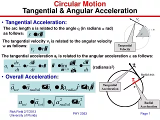
1. 7.4 Angular Acceleration There is in fact a second type of acceleration (in addition to centripetal acceleration) that can be associated with circular motion. Angular acceleration occurs when the circular motion is not uniform; that is, if the tangential speed is increasing or decreasing. In the last lecture, we often referred to a merry-go-round or a turntable. These undergo UCM most of the time, but at some point they have to come to a stop and then start up again. During these periods of time, they have a non-zero angular acceleration. Average angular acceleration is, not surprisingly, (that’s a Greek lower-case “alpha”).
2. 7.4 Angular Acceleration In most cases, we are only concerned with constant angular acceleration. Then if at t = 0, we can write or (note the resemblance to the translational case from chapter 2, where and ). As with arc length and angle (), and tangential and angular speeds (), we can relate the tangential acceleration to the angular acceleration:. In the text (and the notes from last class), we dropped the subscript on the tangential speed , since this is the onlypossible type of speed involved with circular motion. We can not do the same thing here, since we must distinguish from .
3. 7.4 Angular Acceleration Note carefully that centripetal acceleration is necessary for circular motion, but tangential acceleration is not. The two acceleration vectors are perpendicular to each other at any moment, and the total acceleration vector is , where and are unit vectors in the tangential and radial directions. The table shown here illustrates similarities between translational and angular motion.
4. Problem #1: Fan Blades WBL EX 7.49 The blades of a fan running at low speed turn at 250 rpm. When the fan is switched to high speed, the rotation rate increases uniformly to 350 rpm in 5.75 s. What is the magnitude of the angular acceleration of the blades? How many revolutions do the blades go through while the fan is accelerating? Solution: In class
5. Problem #2: Dizzy Hamster The hamster shown in this video has decided to undergo some nonuniform circular motion (FOR SCIENCE!) Let’s analyze the hamster’s kinematics during the time it’s spinning. The hamster’s name is Steve. Steve starts spinning at the 31-second mark of the video and falls out at the 36-second mark. During this time, Steve’s angular velocity decreases in magnitude from 25.0 rad/s to 12.5 rad/s. We will assume that the angular acceleration is constant during this time and that Steve’s 0.15-kg body exists entirely at a radius of 5 cm. What are the signs of ωand α? What is the constant angular acceleration, α? How many revolutions does Steve make? What is the total distance that Steve travels while he is spinning? What is Steve’s maximum tangential speed? What is the largest magnitude of centripetal acceleration that Steve experiences? What is the largest magnitude of centripetal force that Steve experiences?
6. 7.5 Newton’s Law of Gravitation At this point in the course, our knowledge of gravity is simply that “it produces an acceleration of magnitude 9.80 m/s, directed downward”, and that “this magnitude depends weakly on one’s location on the surface of the Earth, and that it doesn’t change much up to altitudes of 100 km or so”. That second statement is a bit annoying. Why should classical mechanics produce results that are only valid in particular regions of the universe? Well…it doesn’t. Newton’s Universal Law of Gravitation tells us what sort of gravitational forces are present among any masses at any distances from each other. It’s valid for planets, moons, stars, and even galaxies.
7. 7.5 Newton’s Law of Gravitation The law provides a relationship for the gravitational interaction between two point masses and , separated by a distance r. It states that every particle in the universe has an attractive gravitational interaction with every other particle in the universe. These forces of mutual interaction are equal and opposite Newton’s 3rd-law pairs (). Furthermore, the law states that the magnitude of the gravitational force depends inversely on the square of the distance between the masses (inverse-square forces tend to be rather prominent in universes with three spatial dimensions). Finally, the force depends on the product of the two masses themselves.
8. 7.5 Newton’s Law of Gravitation All together, we can write Newton’s law of gravitation mathematically as , . ( is called the universal gravitational constant). From the 1/r2 dependence, we see that not only is gravity a non-contact force, it acts over an infinitely long range. Masses that are separated by hundreds of billions of km still exhibit a gravitational attraction, albeit a weak one.
9. 7.5 Newton’s Law of Gravitation Of course, most interesting masses are not point masses; they have a spatial extent. For homogeneous spheres, the preceding equation is valid if we consider all of the mass to exist at the center of the sphere (and if we only wish to calculate outside of the spheres’ surfaces). Proving this requires calculus, but the figure should at least convince you that the direction of makes sense. It should be noted that Newton didn’t have a good way of determining the value of the proportionality constant . It was first measured by Henry Cavendish about 100 years after Newton first published the inverse-square law.Even today, remains one of the “least-precise” physical constants. Some physicists would argue that even the three significant digits shown on the previous slide are one too many.
10. 7.5 Newton’s Law of Gravitation Well, now we have two equations for the gravitational force: and How are they related? Let’s assume that the two masses are a (relatively small mass) and (a planet’s mass) . Newton’s 2nd law can then be used to analyze the acceleration of due to the gravitational force: Thus, the acceleration due to gravity at any distance from the planet’s center (assuming that it’s outside of the planet’s surface) is
11. 7.5 Newton’s Law of Gravitation What if this acceleration is being measured by someone at the Earth’s surface? In this case, (the mass of the Earth), and (the radius of the Earth). Plugging in the numbers, we get This is the value of g that we have been using since chapter 2. Well, almost. We use 9.80. There’s various reasons – primarily, the fact that the Earth isn’t perfectly spherical, so the value of shown above is just an approximation. Note that our equation for does not involve m, the mass of the object. This agrees with our experimental observation that acceleration due to free-fall is independent of the mass of the falling object.
12. 7.5 Newton’s Law of Gravitation We are now in a position to calculate the magnitude of gravitational acceleration at higher altitudes. If h is the altitude, then the distance from the Earth’s center is , and Since 6370 km, an altitude of a few hundred km is required in order to achieve a noticeable change in . Later, we will learn why astronauts appear “weightless”, despite the data below.
13. 7.5 Newton’s Law of Gravitation In chapter 5, we learned that an object at a height h above a (zero-potential-energy) reference level has a potential energy . However, this was valid only if the gravitational force was constant over the distance h. As we now know, if h is very large, Fgis not constant; it varies with position. Using fairly simple calculus (not repeated here), it can be shown that the gravitational potential energy of two point masses separated by a distance r is (this definition requires that we set U = 0 when the objects are infinitely far apart; i.e. ). If we consider a mass m at an altitude of h above the Earth’s surface, then
14. 7.5 Newton’s Law of Gravitation We say that the Earth (in fact, any mass) exists in a negative gravitational potential energy well. As h increases, U becomes less negative. Thus, when gravity does negative work (an object moves higher in the well) or positive work (an object falls lower in the well), there is a change in potential energy. This energy change will be beneficial in solving some upcoming problems. Our equation for Ucan also be extended to the case of three or more masses. For example,
15. 7.5 Newton’s Law of Gravitation For example, when considering the total mechanical energy of a mass m1 in orbit about a mass m2, we have . Rearranging, we have Although we like to think that the Earth’s orbit about the sun is circular, it is actually slightly elliptical (more on that later). At perihelion (the point of closest approach), the speed of the Earth in its orbit is slightly faster than at aphelion (the farthest point).
16. Problem #3: High-Altitude Gravitational Acceleration WBL LP 7.17
17. Problem #4: Orbit of the Moon WBL EX 7.59/7.63 The moon orbits the Earth with an approximately circular orbit of radius 3.85 x 105 km, and an orbital period of 27.5 days. Use this data to calculate the mass of the Earth What is the moon’s tangential speed? What is the moon’s kinetic energy? What is the Earth-moon system’s potential energy? What is the system’s total energy? Solution: In class
18. Problem #5: Gravitational Potential Energy WBL EX 7.64 What is the gravitational potential energy of the configuration shown in the figure, if all of the masses are 1.0 kg? What is the gravitational force per unit mass at the center of the configuration? Solution: In class
19. 7.6 Kepler’s Laws and Earth Satellites In the very early 1600s (pre-dating Newton), Johannes Keplerproduced three empirical laws that governed planetary motion. With the benefit of Newton’s law of gravitation, Kepler’s laws can now be derived using just a few lines of algebra. We present the laws here. Note that they do not only apply to planetary orbits. Any system consisting of a body revolving about a much more massive body due to an inverse-square force conforms to Kepler’s laws.
20. 7.6 Kepler’s Laws and Earth Satellites Kepler’s First Law (the law of orbits) Planets move in elliptical orbits, with the sun at one of the focal points. This fact was alluded to a few slides ago. Absolutely nothing about Newton’s Law of Gravitation suggests that the orbits need to be circular; the orbits are in fact ellipses (at least in the case of closed orbits. For open orbits, in which a body approaches the sun and then leaves, never to return, the path is a hyperbola or parabola). As you may recall, a circle is a special case of ellipse for which the two focal points coincide. Most planets have orbits that are nearly circular; the Earth’s perihelion and aphelion differ by only about 3% of the average Earth-sun separation.
21. 7.6 Kepler’s Laws and Earth Satellites Kepler’s Second Law (the law of areas) A line from the sun to a planet sweeps out equal areas in equal times. This is illustrated in the figure below. Since the speed of the planet is greatest when it is closer to the sun (slide 15), the arc lengths and swept out during the same time duration are not equal in length. However, the two areas and are equal. This can be proven fairly easily using techniques from chapter 8, but we won’t attempt it here.
22. 7.6 Kepler’s Laws and Earth Satellites Kepler’s Third Law (the law of periods) The square of the orbital period of a planet is directly proportional to the cube of the average distance of the planet from the sun. That is, This law can be proven fairly easily in the special case of a circular orbit. Since the centripetal force is supplied by the force of gravity, these forces are equal. Using Ms and mp as the masses of the sun and the planet, respectively, and thus the speed of the orbiting planet (constant, in a circle) is
23. 7.6 Kepler’s Laws and Earth Satellites Kepler’s Third Law (the law of periods) cont’ However, we also know from last lecture that the speed is related to the period as . Therefore, Squaring both sides and solving for T gives Which is a mathematical statement of the law. It’s important to note that the proportionality constant (the term in the brackets) depends only on the sun’s mass. In this way, we can easily calculate the masses of various planets by observing the orbital radii and periods of their moons.
24. 7.6 Kepler’s Laws and Earth Satellites Kepler’s Third Law (the law of periods) cont’ This law can be used to determine the required orbital altitude of a geosynchronous satellite. This is a satellite whose orbital period is one day, such that it’s always overhead of the same point on the Earth’s surface†. These orbits are useful for communications satellites, since the relay stations on the Earth’s surface don’t have to continuously re-aim. A good example can be found on p. 242 of the text. † I’ve skipped a whole lot of physics here. A geosynchronous satellite can only remain overhead of the same point on the Earth’s surface if that point lies on the equator – this is called a geostationary orbit. A geosynchronous orbit that isn’t geostationary does move relative to this point during each day, but not by a large degree.
25. 7.6 Kepler’s Laws and Earth Satellites Earth’s Satellites We conclude this chapter with a few words about man-made satellites and the physics that governs their flight and orbits. First, consider this “thought experiment”. From chapter 2, we know that when an object is projected upward, it slowly loses speed (since acceleration is downward). Eventually, it will come to an instantaneous stop, after which it will fall back downward (accelerating as it goes). In this case, we assumed that the acceleration was constant. What if acceleration became weaker as the object climbed to higher altitudes? Is it possible for the object to have a sufficiently high initial speed for it to “outrun” the weakening acceleration, such that it never comes to a stop? The answer is yes!
26. 7.6 Kepler’s Laws and Earth Satellites Earth’s Satellites cont’ We can show this using conservation of energy. Suppose that a spacecraft is initially on the surface of the Earth, and that it is given a speed which is sufficient for it to escape the Earth’s potential well – that is, it only slows to a stop when it is infinitely far away. Conservation of energy tells us that In this case, (the terminology will become clear in a moment), and . Furthermore, (why?) Rearranging, we find that
27. 7.6 Kepler’s Laws and Earth Satellites Earth’s Satellites cont’ is called the escape speed (roughly 11.2 km/s) - the initial speed needed to escape from the surface of the Earth (without falling back toward it). It depends only on the Earth’s parameters, not those of the spacecraft. Of course, we can calculate escape speeds from any other planet / moon / asteroid / etc., as long as we know its mass and radius.
28. 7.6 Kepler’s Laws and Earth Satellites Earth’s Satellites - Tangential Speed and “Zero-Gravity” Earlier in this lecture, we saw that m/s2 at the altitude of the space shuttle (≈ 400 km). This may seem strange, because video of astronauts aboard the shuttle seems to show that they are weightless. What’s going on here? Remember that any orbiting body must have a tangential speed – if we simply placed the space shuttle at an altitude of 400 km and released it, it would come plummeting back to Earth. The tangential speed depends on the desired orbital altitude. Recycling our Kepler’s 3rd law math, (as usual, r is the distance from the center of the Earth).
29. 7.6 Kepler’s Laws and Earth Satellites Earth’s Satellites - Tangential Speed and “Zero-Gravity” cont’ This tangential speed sees to it that the satellite continuously “falls” around the Earth. If an insufficient tangential speed is reached, the satellite will spiral inward toward the Earth, eventually burning up in the atmosphere (due to the rather extreme drag force…kinetic energy is converted to thermal energy!). If the tangential speed is too great, the satellite simply achieves an elliptical orbit. If , the satellite leaves its orbit and moves off into space.
30. 7.6 Kepler’s Laws and Earth Satellites Earth’s Satellites - Tangential Speed and “Zero-Gravity” cont’ The reason that astronauts aboard the space shuttle appear to be weightless is simply that the shuttle and its occupants are accelerating toward the Earth at the same rate. It’s the same effect that would occur if a person was inside an elevator when the cable snapped. The effect can be safely replicated near the Earth’s surface in an airplane that flies in a parabolic arc (or unsafely replicated in an airplane that has stalled!)
31. Problem #6: Kepler Orbits WBL LP 7.19
32. Problem #7: Satellite About Venus WBL EX 7.71 Venus has a rotational period of 243 days and a mass of 4.87 x 1024 kg. What would be the altitude of a “venosynchronous” satellite? Solution: In class
33. Problem #8: Asteroid Belt WBL EX 7.69 The asteroid belt that lies between Mars and Jupiter may be the debris of a planet that broke apart, or that was not able to form as a result of Jupiter’s strong gravitation. An average asteroid in the belt has an orbital period (about the sun) of about 5.0 years. Approximately how far from the sun would this “fifth” planet have been? Solution: In class