Understanding the Syntax of Programming Language L: Variables, States, and Instructions
220 likes | 375 Vues
This text provides a detailed mathematical description of the programming language L, focusing on its syntax, including input and local variables, output variables, labels, statements, and program structure. It explains concepts such as instruction types, program states, snapshots of execution, and the process of computation within L. Through examples and case analyses, the document outlines how variables assume different values during execution and the importance of program states in understanding the flow of execution.

Understanding the Syntax of Programming Language L: Variables, States, and Instructions
E N D
Presentation Transcript
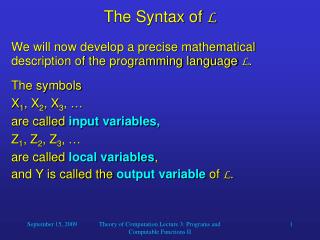
The Syntax of L • We will now develop a precise mathematical description of the programming language L. • The symbols • X1, X2, X3, … • are called input variables, • Z1, Z2, Z3, … • are called local variables, • and Y is called the output variable of L. Theory of Computation Lecture 3: Programs and Computable Functions II
The Syntax of L • The symbols • A1, B1, C1, D1, E1,A2, B2, C2, … • are called labels of L. • For variables and labels, the subscript 1 can always be omitted. Theory of Computation Lecture 3: Programs and Computable Functions II
The Syntax of L • A statement is one of the following: • V V+1 • V V-1 • V V • IF V0 GOTO L • Here, V may be any variable and L may be any label. • Note that the statement V V leaves all values unchanged, so it is a “dummy” command. • We will later see why it is useful to have V V in our set of statements. Theory of Computation Lecture 3: Programs and Computable Functions II
The Syntax of L • An instruction is either • a statement (unlabeled instruction) or • [L] followed by a statement (instruction labeled L) • A program is a list (i.e., a finite sequence) of instructions. • The length of this list is called the length of the program. • We also include the empty program – the program of length 0 – in the set of all programs. Theory of Computation Lecture 3: Programs and Computable Functions II
The Syntax of L • While a program is being executed, its variables assume different numerical values. • This motivates the concept of the state of a program: • A state of a program P is a list of equations of the form • V = m, • where V is a variable and m is a number, • including exactly one equation for each variable that occurs in P (and possibly equations for other variables). Theory of Computation Lecture 3: Programs and Computable Functions II
The Syntax of L Is the list X = 4, Y = 3, Z = 3a state of P ? • Consider the following program P : • [A] IF X0 GOTO B • Z Z+1 • IF Z0 GOTO E • [B] X X-1 • Y Y+1 • Z Z+1 • IF Z0 GOTO A Yes. How about X1 = 4, X2 = 5, Y = 4, Z = 4? Yes. And X = 3, Z = 3? No. Theory of Computation Lecture 3: Programs and Computable Functions II
The Syntax of L • Let be a state of P and let V be a variable that occurs in . • The value of V at is then the unique number q such that the equation V = q is one of the equations in . • For example, the value of X at the stateX = 4, Y = 3, Z = 3 • is 4. Theory of Computation Lecture 3: Programs and Computable Functions II
The Syntax of L • Consider a machine that can execute programs of L. • During program execution, this machine needs to store the state of a program, i.e., keep track of the values of variables. • Is there anything else that needs to be stored? • Yes, we also need to store which instruction is to be executed next. Theory of Computation Lecture 3: Programs and Computable Functions II
The Syntax of L • Therefore, we define a snapshot or instantaneous description of a program P of length n to be a pair (i, ) where 1 i (n + 1), and is a state of P. • The number i indicates the number of the instruction that is to be executed next. • i = n + 1 corresponds to a “stop” instruction. • A snapshot (i, ) of a program P of length n is called terminal if i = n + 1. • If s = (i, ) is a snapshot of P and V is a variable of P , then the value of V at s just means the value of V at . Theory of Computation Lecture 3: Programs and Computable Functions II
The Syntax of L • If (i, ) is a nonterminal snapshot of P , we define the successor of (i, ) to be the snapshot (j, ) defined as follows: • Case 1: • The i-th instruction of P is V V+1 and contains the equation V = m. • Then j = i + 1 and is obtained from by replacing the equation V = m by V = m + 1(the value of V at is m + 1). Theory of Computation Lecture 3: Programs and Computable Functions II
The Syntax of L • Case 2: • The i-th instruction of P is V V-1 and contains the equation V = m. • Then j = i + 1 and is obtained from by replacing the equation V = m by V = m – 1 if m 0. • If m = 0, then = . • Case 3: • The i-th instruction of P is V V. • Then j = i + 1 and = . Theory of Computation Lecture 3: Programs and Computable Functions II
The Syntax of L • Case 4: • The i-th instruction of P is IF V0 GOTO L. • Then = and there are two subcases: • Case 4a: • contains the equation V = 0. • Then j = i + 1. • Case 4b: • contains the equation V = m where m 0. • Then, if there is an instruction of P labeled L, j is the least number such that the j-th instruction of P is labeled L. Otherwise, j = n + 1. Theory of Computation Lecture 3: Programs and Computable Functions II
The Syntax of L • A computation of a program P is defined to be a sequence s1, s2, …, sk of snapshots of P such that si+1 is the successor of si for i = 1, 2, …, k – 1 and sk is terminal. Theory of Computation Lecture 3: Programs and Computable Functions II
Computable Functions • What does it exactly mean when we say that a program computes a function? • We would like to find a precise definition for this. • Let P be any program in the language L and let r1, …, rm be m given numbers. • We form the state of P which consists of the equations • X1 = r1, X2 = r2, …, Xm = rm, Y = 0together with the equations V = 0 for all other variables V in P. • We call this the initial state. Theory of Computation Lecture 3: Programs and Computable Functions II
Computable Functions • Moreover, we call the snapshot (1, ) the initial snapshot. • When running the program, there are two possible outcomes: • Case 1: • There is a computation s1, s2, …, sk of P beginning with the initial snapshot. • Then we write P(m)(r1, r2, …, rm) for the value of the variable Y at the terminal snapshot sk. Theory of Computation Lecture 3: Programs and Computable Functions II
Computable Functions • Case 2: • There is no such computation; i.e., there is an infinite sequence s1, s2, s3, …beginning with the initial snapshot. • In this case, P(m)(r1, r2, …, rm) is undefined. Theory of Computation Lecture 3: Programs and Computable Functions II
Sample Computation [A] IF X0 GOTO B (1) Z Z+1 (2) IF Z0 GOTO E (3) [B] X X-1 (4) Y Y+1 (5) Z Z+1 (6) IF Z0 GOTO A (7) • (1, {X = r, Y = 0, Z = 0}), • (4, {X = r, Y = 0, Z = 0}), • (5, {X = r - 1, Y = 0, Z = 0}), • (6, {X = r - 1, Y = 1, Z = 0}), • (7, {X = r - 1, Y = 1, Z = 1}), • (1, {X = r - 1, Y = 1, Z = 1}), • . • . • (1, {X = 0, Y = r, Z = r}), • (2, {X = 0, Y = r, Z = r}), • (3, {X = 0, Y = r, Z = r + 1}), • (8, {X = 0, Y = r, Z = r + 1}). We write: P(1)(r) = r. Theory of Computation Lecture 3: Programs and Computable Functions II
Computation • For any program P and any positive integer m, the function P(m)(r1, r2, …, rm) is said to be computed by P. • We allow any program to be run with any number of inputs. • Consider the summation program from the previous lecture: • P(2)(r1, r2) = r1 + r2 • P(1)(r1) = r1 + 0 = r1 • P(3)(r1, r2 ,r3) = r1 + r2 Theory of Computation Lecture 3: Programs and Computable Functions II
Computation • For any program P and any positive integer m, the function P(m)(r1, r2, …, rm) is said to be computed by P. • In general, a partial function f on a set Sm is a function whose domain is a subset of Sm. • If a partial function on Sm has the domain Sm, then it is called total. Theory of Computation Lecture 3: Programs and Computable Functions II
Computation • A given partial function g (of one or more variables) is said to be partially computable if it is computed by some program. • This is the case if there is a program P such that • g(r1, r2, …, rm) = P(m)(r1, r2, …, rm) for all r1, r2, …, rm. • This means not only that both sides have the same value when they are defined, but also that when either side of the equation is undefined, the other one is as well. • A function is said to be computable if it is both partially computable and total. Theory of Computation Lecture 3: Programs and Computable Functions II
Macros • So far we have used macros in an informal way. Let us now develop a more precise definition of them. • Let f(x1, x2, …, xn) be a partially computable function, and P be a program that computes f. • Let us assume that • the variables in P are named Y, X1, …, Xn, Z1, …, Zk, • the labels in P are named E, A1, …, Al, and • for each instruction of P of the form IF V0 GOTO Ai there is in P an instruction labeled Ai . Theory of Computation Lecture 3: Programs and Computable Functions II
Macros • We can modify any program of the language L to comply with these assumptions. • We write: • P = P (Y, X1, …, Xn, Z1, …, Zk; E, A1, …, Al) • In particular, we will use: • Qm = P (Zm, Zm+1, …, Zm+n, Zm+n+1, …, Zm+n+k; Em, Am+1, …, Am+l) • for a given value m. Theory of Computation Lecture 3: Programs and Computable Functions II