Download

1 / 32
320 likes | 458 Vues
Bayesian Analysis and Applications of A Cure Rate Model. Introduction. Standard Cure Rate Model: : represents the survivor function for the entire population. : represents the survivor function for the non-cured

E N D
Introduction • Standard Cure Rate Model: : represents the survivor function for the entire population. : represents the survivor function for the non-cured group in the population. Exponential and Weibull distributions are commonly used : means the cured population.
Drawbacks 1. Cannot have a proportional hazard structure 2. When including covariates through the parameter via a standard binomial regression model, the standard cure rate model yields improper posterior distributions. Then it implies that Bayesian inference with a standard cure rate model essentially requires a proper prior.
New Model • N denote the number of cancer cells left active for that individual after the initial treatment, and have a Poisson distribution with mean • denotes the random time for the ith cancer cell to produce a detectable cancer mass and assumed them to be iid with a common distribution function F ( t ) = 1- S ( t ) and be independent of N. • Y= min ( , ) denotes the time to relapse of the cancer, where P ( ) =1. • Hence, the survival function for the population is given by = P ( no cancer by time y) =P ( N = 0 ) + P ( ) =exp( - F(y)).
Property of the New Model • , the cure rate fraction, is not a proper model. As , the cure fraction tends to 0, whereas as the cure fraction tends to 1. • The density function The hazard function: They are not proper probability density function or hazard function. However is multiplicative in and f(y); thus, it has the proportional hazard structure which is more appealing than the one from the standard cure rate model and is computationally attractive.
Property of the New Model(Con.) • The model can be written as: where which is a proper survival function. The density function is and the hazard function is: which doesn’t have a proportional hazard structure. It shows a mathematical relationship between the standard cure rate model and the new model. • In this model, let ,where x is a vector of covariates and is vector of regression coefficients.
The Likelihood Function • Let n be the number of subjects. be the failure time for the ith subject. be the censoring time. be the censoring indicator. ‘1’ means failure time, ’0’ means right censoring. be the observed data, be the total data. N be an unobserved vector of a latent variable be the number of carcinogenic cells for the ith subject, assuming that are Poisson random variables with mean , i=1,2,…..,n.
The Likelihood Function(Con.) • Suppose that the iid incubation times for the cancer cells for the ith subject and all have cdf • The complete-data likelihood function of the parameter is Where
The Likelihood Function(Con.) • By summing out the unobserved latent vector N, the complete-data likelihood function can be reduced to
The Noninformative Prior Distibution • Suppose a joint noninformative prior for of the form where are the parameters in . This noninformative prior implies that and are independent priors and that is a uniform improper prior. Then, the posterior distribution of based on the observed data is given follows log-logistic, Gompertz and gamma distributions , respectively
The Noninformative Prior Distibution(Con.) • Even though we consider three distributions for , we give the same conditions which are where and are two specified hyperparameters. • Let and be an matrix with rows . If (a) is of full rank, (b) is proper, (c) and , • Based on these condition, we can get the result which is that the posterior is proper.
The Noninformative Prior Distibution(Con.) • Based on the specific property for Gompertz distribution, we can have another conditions and still get the same results. Firstly, we assume throughout that where and are two specified hyperparameters, where and , the posterior distribution of based on the observed data is Secondly, let and be an matrix with rows . If (a) is of full rank, (b) is proper, (c) and , where . Then the posterior is proper.
The Informative Prior Distibution • Kolmogorov-Smirnov Test To determine if two datasets differ significantly The Kolmogorov-Smirnov two sample test statistic is defined as where E1 and E2 are the empirical distribution functions based on Kaplan-Meier survival estimate for the two samples.
The Informative Prior Distibution • is an matrix of covariates corresponding to , let denote the complete historical data. Further, let denotes the initial prior distribution for We propose a joint informative prior distribution of the form where is the complete data likelihood with D being replaced by the historical data and We take a noninformative prior for such as , which implies . A beta prior is chosen for leading to the joint prior distribution. where are the specified prior parameters
Data Analysis • We will demonstrate the application of our proposed models by analyzing the data from a phase III melanoma clinical trial. 1. Observe the maximum likelihood estimates of the parameters for the proposed models under three different distributions. 2. Carry out a Bayesian analysis with covariates using the proposed noninformative priors. In this study, we obtain the posterior estimates of the parameters for the proposed models with log- logistic, Gompertz and gamma distributions. 3. Carry out a Bayesian analysis with covariates using the proposed informative priors. Three covariates are included in the analyses, they are age ( ), gender ( : male, female), and performance status (PS) ( : fully active, other)
Data Analysis(Con.) • Summary of E1684 data Survival time (year) Median 2.91 SD 2.83 Status(frequency) Censored 110 Death 174 Age(year) Mean 47.03 SD 13.00 Gender(frequency) Male 171 Female 113 PS (frequency) Fully active 253 Other 31
Data Analysis(Con.) • Summary of E 1673 data Survival time (year) Median 5.72 SD 8.20 Status(frequency) Censored 257 Death 393 Age(year) Mean 48.02 SD 13.99 Gender(frequency) Male 375 Female 275 PS (frequency) Fully active 561 Other 89
Data Analysis(Con.) • Figure 1.1 displays a Kaplan-Meier plot for overall survival. The three different distributions fit the data all well.
Data Analysis (Con.) • MLE's of the model parameters for the E1684 data Compare with the maximum likelihood estimates, standard deviations and p-values for the proposed models under log-logistic, Gompertz, and Gamma distributions each other. We find that all results are similar. The p-values associated with the covariates are all greater than 0.05. This implies that none of age, gender and PS is statistically significant at level =0.05.
Data Analysis (MLE Analysis) • The following is the MLE's of the Model Parameters with Weibull Distribution • Variable MLE SD P-value Age 0.06 0.04 0.12 Gender -0.15 0.12 0.22 PS -0.20 0.26 0.44 1.31 0.09 0.00 -1.34 0.12 0.00
Data Analysis (MLE Analysis) • The following is the MLE's of the Model Parameters with log-logistic Distribution • Variable MLE SD P-value Age 0.07 0.04 0.06 Gender -0.13 0.12 0.31 PS -0.20 0.26 0.44 1.61 0.13 0.00 -1.28 0.16 0.00
Data Analysis (MLE Analysis) • The following is the MLE's of the Model Parameters with Gompertz Distribution • Variable MLE SD P-value Age 0.06 0.04 0.12 Gender -0.15 0.12 0.22 PS -0.20 0.26 0.43 0.27 0.03 0.00 -1.97 0.19 0.00
Data Analysis (MLE Analysis) • The following is the MLE's of the Model Parameters with Gamma Distribution • Variable MLE SD P-value Age 0.06 0.04 0.12 Gender -0.15 0.12 0.22 PS -0.20 0.26 0.44 1.56 0.12 0.00 -0.51 0.14 0.00
Data Analysis (Noninfroamtive and Informative Prior Analysis) • We carry out a Bayesian analysis with covariates using the proposed noninformative or informative priors to demonstrate our second or third application of the proposed model under the three different distributions. E1684 is used as current data. , we take an improper uniform prior, and for , we take =1 and =0.01 to ensure a proper prior.The parameter is taken to have a normal distribution with mean 0 and variance 10,000. E1673 serves as the historical data for our Bayesian analysis of E1684.
Data Analysis (Result) • Incorporating historical data can yield more precise posterior estimates for age, gender and PS. Their posterior estimates, SD, and 95% HPD do not change a great deal if a low or moderate weight is given to the historical data. However, if a higher than moderate weight is given, the posterior summaries can change substantially. Then, age and gender are potentially important factors for predicting survival.The posterior estimate for age is positive, implying that as age goes up, the number of carcinogenic cells increases. Therefore, older patients have shorter relapse-free survival. the posterior estimate of gender is negative, implying that the number of carcinogenic cells for females are less than the number of carcinogenic cells for males.
Data Analysis (Result) • as the posterior estimate of increases, the posterior estimate for age becomes larger while the posterior estimates for gender and PS become smaller. The posterior standard deviations of the model parameters become smaller and the 95% HPD become narrower as the posterior estimate of increases. This demonstrates that incorporation of historical data can yield precise posterior estimates of age, gender and PS parameters. We can see that there is a large difference in these estimates, especially in the standard deviations and 95% HPD.
Data Analysis (Result) • When a low weight is given to the historical data, the posterior estimate of PS is negative. It implies that cancer cell counts for the patients whose PS is fully active are more than that when PS is not fully active after the initial treatment. When a higher weight is given to the historical data, the posterior estimate of PS becomes positive which implies that patients whose PS is fully active have longer relapse-free survival than patients whose PS is not fully active. The posterior estimates for age are all positive and their values increase when the posterior estimate of increases. This implies that as age goes up, the number of carcinogenic cells increases. This tells us that incorporation historical data, we can obtain better results. The posterior estimates for gender are all negative and becomes smaller when the power is increasing. There is a gender difference, when we incorporate historical data, the difference becomes significant.
Data Analysis (Detailed Sensitivity Analysis by Varying the Hyperparameters) • For illustration purposes, we only show results with a fixed value for . In our study, we fix the hyperparameters for =0.29and vary the hyperparameters for . Firstly, varying the variance of and from small value to large value which implies that shape of the or becomes from narrow to flat. Secondly, varying the mean of or from the small to large. Based on the two conditions, we check the influence on the regression coefficients. Through these detailed sensitivity analysis, we find that the posterior estimates of age, gender and PS are robust for a wide range of hyperparameter values.
Conclusion and Discussion • We have also investigated the melanoma data using three different methods for each distribution: Even though we use different methods and different distributions, the results are almost the same. Incorporation of historical data can improve the posterior estimates, standard deviations and 95% HPD of age, gender and PS. And age and gender are potentially important prognostic factors for predicting overall survival in melanoma. This demonstrates a desirable feature of our model. Such a conclusion is not possible based only on a frequentist or a Bayesian analysis of the current data alone. Thus, incorporating historical data can yield more precise posterior estimates of age, gender and PS.