Download

1 / 45
450 likes | 691 Vues
Production Planning & Scheduling in Large Corporations. Dealing with the Problem Complexity through Decomposition. Corporate Strategy. Aggregate Unit Demand. Aggregate Planning. (Plan. Hor.: 1 year, Time Unit: 1 month). Capacity and Aggregate Production Plans. End Item (SKU) Demand.

E N D
Dealing with the Problem Complexity through Decomposition Corporate Strategy Aggregate Unit Demand Aggregate Planning (Plan. Hor.: 1 year, Time Unit: 1 month) Capacity and Aggregate Production Plans End Item (SKU) Demand Master Production Scheduling (Plan. Hor.: a few months, Time Unit: 1 week) SKU-level Production Plans Manufacturing and Procurement lead times Materials Requirement Planning (Plan. Hor.: a few months, Time Unit: 1 week) Component Production lots and due dates Shop floor-level Production Control Part process plans (Plan. Hor.: a day or a shift, Time Unit: real-time)
Product Aggregation Schemes • Items (or Stock Keeping Units - SKU’s):The final products delivered to the (downstream) customers • Families: Group of items that share a common manufacturing setup cost; i.e., they have similar production requirements. • Aggregate Unit:A fictitious item representing an entire product family. • Aggregate Unit Production Requirements: The amount of (labor) time required for the production of one aggregate unit. This is computed by appropriately averaging the (labor) time requirements over the entire set of items represented by the aggregate unit. • Aggregate Unit Demand: The cumulative demand for the entire set of items represented by the aggregate unit. Remark:Being the cumulate of a number of independent demand series, the demand for the aggregate unit is a more robust estimate than its constituent components.
Computing the Aggregate Unit Production Requirements Aggregate unit labor time = (.32)(4.2)+(.21)(4.9)+(.17)(5.1)+(.14)(5.2)+ (.10)(5.4)+(.06)(5.8) = 4.856 hrs
Aggregate Planning Problem Aggr. Unit Production Reqs Corporate Strategy Aggregate Unit Demand Aggregate Production Plan Aggregate Planning Aggregate Unit Availability (Current Inventory Position) Required Production Capacity • Aggregate Production Plan: • Aggregate Production levels • Aggregate Inventory levels • Aggregate Backorder levels • Production Capacity Plan: • Workforce level(s) • Overtime level(s) • Subcontracted Quantities
PC WC HC FC D(t) P(t) = D(t) W(t) Pure Aggregate Planning Strategies 1.Demand Chasing: Vary the Workforce Level • D(t): Aggregate demand series • P(t): Aggregate production levels • W(t): Required Workforce levels • Costs Involved: • PC: Production Costs • fixed (setup, overhead) • variable (materials, consumables, etc.) • WC: Regular labor costs • HC: Hiring costs: e.g., advertising, interviewing, training • FC: Firing costs: e.g., compensation, social cost
Pure Aggregate Planning Strategies 2.Varying Production Capacity with Constant Workforce: PC SC WC OC UC D(t) P(t) S(t) O(t) U(t) W = constant • S(t): Subcontracted quantities • O(t): Overtime levels • U(t): Undertime levels • Costs involved: • PC, WC: as before • SC: subcontracting costs: e.g., purchasing, transport, quality, etc. • OC: overtime costs: incremental cost of producing one unit in overtime • (UC: undertime costs: this is hidden in WC)
PC WC IC D(t) P(t) I(t) W(t), O(t), U(t), S(t) = constant Pure Aggregate Planning Strategies 3.Accumulating (Seasonal) Inventories: • I(t):Accumulated Inventory levels • Costs involved: • PC, WC:as before • IC:inventory holding costs: e.g., interest lost, storage space, pilferage, obsolescence, etc.
Pure Aggregate Planning Strategies 4.Backlogging: PC WC BC D(t) P(t) B(t) W(t), O(t), U(t), S(t) = constant • B(t):Accumulated Backlog levels • Costs involved: • PC, WC:as before • BC:backlog (handling) costs: e.g., expediting costs, penalties, lost sales (eventually), customer dissatisfaction
Typical Aggregate Planning Strategy A “mixture” of the previously discussed pure options: PC WC HC FC OC UC SC IC BC P W D H F O Io U S I Wo B + • Additional constraints arising from the company strategy; e.g., • maximal allowed subcontracting • maximal allowed workforce variation in two consecutive periods • maximal allowed overtime • safety stocks • etc.
Demand (vs. Capacity) Options or Proactive Approaches to Aggregate Planning • Influencing demand variation so that it aligns to available production capacity: • advertising • promotional plans • pricing (e.g., airline and hotel weekend discounts, telecommunication companies’ weekend rates) • “Counter-seasonal” product (and service) mixing: Develop a product mix with antithetic (seasonal) trends that level the cumulative required production capacity. • (e.g., lawn mowers and snow blowers) • => The outcome of this type of planning is communicated to the overall aggregate planning procedure as (expected) changes in the demand forecast.
Solution Approaches • Graphical Approaches: Spreadsheet-based simulation • Analytical Approaches: Mathematical (mainly linear programming) Programming formulations
Analytical Approach:A Linear Programming Formulation min TC = St ( PCt*Pt+WCt*Wt+OCt*Ot+HCt*Ht+FCt*Ft+ SCt*St+ICt*It+BCt*Bt ) s.t. • t,(u_l_r)*Pt (s_d)*(w_d)t*Wt+Ot Prod. Capacity: • t, Pt+It-1+St = (Dt-Bt)+Bt-1+It Material Balance: • t, Wt = Wt-1+Ht-Ft Workforce Balance: ( Any additional policy constraints ) Var. sign restrictions: • t, Pt, Wt, Ot, Ht, Ft, St, It, Bt 0 Time unit: month / unit_labor_req. /shift_duration (in hours) / (working_days) for month t
The (Master) Production Scheduling Problem Capacity Consts. Company Policies Product Charact. Economic Considerations Placed Orders MPS Master Production Schedule: When & How Much to produce for each product Forecasted Demand • Current and Planned • Availability, eg., • Initial Inventory, • Initiated Production, • Subcontracted quantities Planning Horizon Time unit Capacity Planning
Grain cracking (1 milling machine) Mashing (1 mashing tun) Boiling (1 brew kettle) Fermentation (3 40-barrel ferm. tanks) Filtering (1 filter tank) Bottling (1 bottling station) MPS Example: Company Operations Fermentation Times:
Inventory Position: IPi = max{IPi-1,0}+ SRi+BNRi -Di (Material Balance Equation) (IPi-1)+ Di i SRi+BNRi IPi Computing Inventory Positions and Net Requirements Net Requirement: NRi = abs(min{0, IPi})
Computing Spoilage and Modified Inventory Position Spoilage: SPi = max{0, IPi-1-(SRi-1+SRi-2+…+SRi-sl+1) -(BNRi-1+BNRi-2+…+BNRi-sl+1)} Inventory Position: IPi = max{IPi-1,0}+ SRi+BNRi -Di-SPi (Material Balance Equation) (IPi-1)+ Di i SPi SRi+BNRi IPi
The Driving Logic behind the Empirical Approach • Initial Inventory Position • Scheduled Receipts due to initiated production or subcontracting Demand Availability: Compute Future Inventory Positions Net Requirements Future inventories Lot Sizing Scheduled Releases Resource (Fermentor) Occupancy Product i Revise Prod. Reqs Feasibility Testing Schedule Infeasibilities Master Production Schedule
MRP Planned Order Releases MPS Current Availabilities Priority Planning The “MRP Explosion” Calculus Lot Sizing Policies Lead Times BOM
Example: The (complete) MRP Explosion Calculus Item BOM: Alpha B(1) C(1) D(2) C(2) E(1) F(1) E(1) F(1) Item Levels: Level 0: Alpha Level 1: B Level 2: C, D Level 3: E, F
The “MRP Explosion” Calculus External Demand Level 0 Capacity Planning Initial Inventories Level 1 Level 2 Scheduled Receipts Level N Planned Order Releases Gross Requirements
Capacity Planning (Example) Available labor hours 150 100 50 8 1 2 3 Periods 4 5 6 7
Computing the item Scheduled Releases Safety Stock Requirements Lot Sizing Policy Lead Time Gross Reqs Planned Order Releases Parent Sched. Rel. Planned Order Receipts Net Reqs Synthesizing item demand series Projecting Inv. Positions and Net Reqs. Lot Sizing Time- Phasing Item External Demand Scheduled Receipts Initial Inventory
Some Lot Sizing Heuristics • Economic Order Quantity (EOQ): Compute a lot size using the EOQ formula with the demand rate D set equal to the average of the demand values observed over the considered planning horizon. • Periodic Order Quantity (POQ): Compute T = round(EOQ/D), and every time you schedule a new lot, size it to cover the net requirements for the subsequent T periods. • Silver-Meal (SM): Every time you start a new lot, keep adding the net requirements of the subsequent periods, as long as the average (setup plus holding) cost per period decreases. • Least Unit Cost (LUC): Every time you start a new lot, keep adding the net requirements of the subsequent periods, as long as the average (setup plus holding) cost per unit decreases. • Part Period Balancing (PPB): Every time you start a new lot, add a number of subsequent periods such that the total holding cost matches the lot set up cost as much as possible.
General Problem Definition Determine the timing of • the releases of the various production lots on the shop-floor and • the allocation to them of the system resources required for the execution of their various operations so that the production plans decided at the tactical planning - i.e., MPS & MRP - level are observed as close as possible.
Example J_2 J_1 W_2 W_i W_1 W_M W_q J_N
A modeling absrtaction • M: number of machine types / workstations. • N: number of jobs to be scheduled. • Job routing: an ordered list / sequence of machines that a job needs to visit in order to be completed. • Operation: a single processing step executed during the job visit to a machine. • P_j: the set of operations in the routing of job j. • t_kj: the processing time for the k-th operation of job j. • d_j: due date for job j. • r_j: the release date of job j, i.e., the date at which the material required for starting the job processing will be available.
Problem variations • Based on job routing: • job shop: each job has an arbitrary route • flow shop: all jobs have the same route, but different operational processing times • re-entrant flow shop: some machine(s) is visited more than once by the same job • flexible job shop / flow shop: each operation has a number of machine alteratives for its execution • Based on the operational processing times: • deterministic: the various processing times are known exactly • stochastic: the processing times are known only in distribution • Based on the possibility of pre-emption: • pre-emptive: the execution of a job on a machine can be interrupted upon the arrival of a new job • non-preemptive: each machine must complete its currently running job before switching to another one. • Based on the considered performance objective(s)
Performance-related job and schedule attributes • job completion time: C_j • schedule makespan: max_j C_j • job lateness: L_j = C_j - d_j (notice that, by definition, job lateness can be either positive or negative - in which case that the job is finished earlier than its due date) • job tardiness: T_j = max (0, L_j) = [L_j]+ • job flow time: F_j =C_j - r_j (i.e., the amount of time the job spends on the shop-floor) • job tardy index: TI_j = 1 if job is tardy; 0 otherwise. • Number of tardy jobs: NT • job importance weight: w_j (the higher the weight, the more important the job)
A feasible schedule and its Gantt Chart Machine 1 2 3 4 5 5 10 15 20 Time Job 1 Job 2 Job 3 Job 4 Job 5
Solution Approaches • Analytical (Mixed Integer Programming) formulations: Notoriously difficult to solve even for relatively small configurations • Heuristics: In thescheduling literature, the applied heuristics are known as dispatching rules, and they determine the sequencing of the various jobs waiting upon the different machines, based upon job attributes like • the required processing times • due dates • priority weights • slack times, defined as d_j - (current time + total remaining processing time) • etc.