Download

1 / 97
1.26k likes | 2.42k Vues
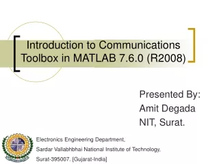
Introduction to Communications Toolbox in MATLAB 7.6.0 (R2008). Presented By: Amit Degada NIT, Surat. Electronics Engineering Department, Sardar Vallabhbhai National Institute of Technology, Surat-395007. [Gujarat-India]. Meaning. Presentation Outline . Objective of the Lecture

E N D
Introduction to Communications Toolbox in MATLAB 7.6.0 (R2008) Presented By: Amit Degada NIT, Surat. Electronics Engineering Department, Sardar Vallabhbhai National Institute of Technology, Surat-395007. [Gujarat-India]
Presentation Outline • Objective of the Lecture • Section Overview • Expected background from the Users • Studying Components of the Communication System • BER : As performance evaluation Technique • Scatter Plot • Simulating a Communication Link….Examples • BERTool : A Bit Error Rate GUI
Objective of The Lecture • Introduce to Communication Toolbox in MATLAB 7.6.0 (R2008) • Cover Basic Expect of Communication system • Exposure to some functions • Simulation analysis of Communication Link • Exposure to Graphical User Interface (GUI) Feature in Communications Toolbox
After The Lecture…….. • You will be able to • Make Communication Link • Analysis of your link with Theoretical Result • For that you have Assignments……..
Presentation Outline • Objective of the Lecture • Section Overview • Expected background from the Users • Studying Components of the Communication System • BER : As performance evaluation Technique • Scatter Plot • Simulating a Communication Link….Examples • BERTool : A Bit Error Rate GUI
Section Overview • Extends the MATLAB technical computing environment with • Functions, • Plots, • And a Graphical User Interface For exploring, designing, analyzing, and simulating algorithms for the physical layer of communication systems • The Toolbox helps you create algorithms for commercial and defense wireless or wireline systems.
Key Features • Functions for designing the physical layer of communications links, including source coding, channel coding, interleaving, modulation, channel models, and equalization • Plots such as eye diagrams and constellations for visualizing communications signals • Graphical user interface for comparing the bit error rate of your system with a wide variety of proven analytical results • Galois field data type for building communications algorithms
Presentation Outline • Objective of the Lecture • Section Overview • Expected background from the Users • Studying Components of the Communication System • BER : As performance evaluation Technique • Scatter Plot • Simulating a Communication Link….Examples • BERTool : A Bit Error Rate GUI
Expected background from User • We assume that you already have the Basic Knowledge of subject called ‘Communication’ • The discussion and examples in this chapter are aimed at New users • Experienced User can go for many online reference that includesinclude examples, a description of the function's algorithm, and references to additional reading material http://www.mathworks.com/matlabcentral/
Presentation Outline • Objective of the Lecture • Section Overview • Expected background from the Users • Studying Components of the Communication System • BER : As performance evaluation Technique • Scatter Plot • Simulating a Communication Link….Examples • BERTool : A Bit Error Rate GUI
Studying Components of Communication system • We will See for two Types: • Analog Communications • Digital Communications
Analog Communication System This may be any analog signal such as Sine wave, Cosine Wave, Triangle Wave………………..
Analog Modulation/Demodulation Functions ammod Amplitude modulation amdemod Amplitude demodulation fmmod Frequency modulation fmdemod Frequency demodulation pmmod Phase modulation pmdemod Phase demodulation ssbmod Single sideband amplitude Mod ssbdemod Single sideband amplitude DeMod
ammod Amplitude modulation Syntax y = ammod(x,Fc,Fs) y = ammod(x,Fc,Fs,ini_phase) y = ammod(x,Fc,Fs,ini_phase,carramp) Where x = Analog Signal Fc = Carrier Signal Fs = Sampling Frequency ini_phase = Initial phase of the Carrier carramp = Carrier Amplitude
amdemod Amplitude Demodulation Syntax z = amdemod(y,Fc,Fs) z = amdemod(y,Fc,Fs,ini_phase) z = amdemod(y,Fc,Fs,ini_phase,carramp) z = amdemod(y,Fc,Fs,ini_phase,carramp,num,den) Where y= Received Analog Signal Fc = Carrier Signal Fs = Sampling Frequency ini_phase = Initial phase of the Carrier carramp = Carrier Amplitude num, den = Coefficients of butterworth low pass filter
Example…….. Amplitude Modulation Generation Fs = 8000; % Sampling rate is 8000 samples per second. Fc = 300; % Carrier frequency in Hz t = [0:.1*Fs]'/Fs; % Sampling times for .1 second x = sin(20*pi*t); % Representation of the signal y = ammod(x,Fc,Fs); % Modulate x to produce y. figure; subplot(2,1,1); plot(t,x); % Plot x on top. subplot(2,1,2); plot(t,y) % Plot y below.
fmmod Frequency modulation Syntax y = fmmod(x,Fc,Fs,freqdev) y = fmmod(x,Fc,Fs,freqdev,ini_phase) Where x = Analog Signal Fc = Carrier Signal Fs = Sampling Frequency ini_phase = Initial phase of the Carrier freqdev = Frequency deviation constant (Hz)
fmdemod Frequency Demodulation Syntax z = fmdemod(y,Fc,Fs,freqdev) z = fmdemod(y,Fc,Fs,freqdev,ini_phase) Where Z = Received Analog Signal Fc = Carrier Signal Fs = Sampling Frequency ini_phase = Initial phase of the Carrier freqdev = Frequency deviation constant (Hz)
pmmod phase modulation Syntax y = pmmod(x,Fc,Fs,phasedev) y = pmmod(x,Fc,Fs,phasedev,ini_phase) Where x = Analog Signal Fc = Carrier Signal Fs = Sampling Frequency ini_phase = Initial phase of the Carrier phasedev = Frequency deviation constant (Hz)
pmdemod phase Demodulation Syntax z = pmdemod(y,Fc,Fs,phasedev) z = pmdemod(y,Fc,Fs,phasedev,ini_phase)) Where x = Analog Signal Fc = Carrier Signal Fs = Sampling Frequency ini_phase = Initial phase of the Carrier phasedev = Frequency deviation constant (Hz)
Example Statement: The example samples an analog signal and modulates it. Then it simulates an additive white Gaussian noise (AWGN) channel, demodulates the received signal, and plots the original and demodulated signals.
Example % Prepare to sample a signal for two seconds, % at a rate of 100 samples per second. Fs = 100; % Sampling rate t = [0:2*Fs+1]'/Fs; % Time points for sampling % Create the signal, a sum of sinusoids. x = sin(2*pi*t) + sin(4*pi*t); Fc = 10; % Carrier frequency in modulation phasedev = pi/2; % Phase deviation for phase modulation y = pmmod(x,Fc,Fs,phasedev); % Modulate. y = awgn(y,10,'measured',103); % Add noise. z = pmdemod(y,Fc,Fs,phasedev); % Demodulate. % Plot the original and recovered signals. figure; plot(t,x,'k-',t,z,'g-'); legend('Original signal','Recovered signal');
Results Fig: Phase modulation and demodulation
Source randintGenerate matrix of Uniformly distributed Random integers randsrcGenerate random matrix using prescribed alphabet randerrGenerate bit error patterns
randint Random Integer Syntax out = randint %generates a random scalar that is either 0 or 1, with equal probability out = randint(m) %generates an m-by-m binary matrix, each of whose entries independently takes the value 0 with probability ½ out = randint(m,n) %generates an m-by-n binary matrix, each of whose entries independently takes the value 0 with probability ½
Example Statement :To generate a 10-by-10 matrix whose elements are uniformly distributed in the range from 0 to 7 out = randint(10,10,[0,7]) or out = randint(10,10,8); Results
Example Statement :How to generate 0s and1s…. out = randint(1,7,[0,1]) Results
Digital Modulation/Demodulation fskmod Frequency shift keying modulation fskdemod Frequency shift keying demodulation pskmod Phase shift keying modulation pskdemod Phase shift keying demodulation mskmod Minimum shift keying modulation mskdemod Minimum shift keying demodulation qammodQuadrature amplitude modulation qamdemodQuadrature amplitude demodulation
fskmod Frequency shift keying modulation Syntax y = fskmod(x,M,freq_sep,nsamp) M is the alphabet size and must be an integer power of 2. The message signal must consist of integers between 0 and M-1. freq_sep is the desired separation between successive frequencies in Hz. nsamp denotes the number of samples per symbol in y and must be a positive integer greater than 1. y = fskmod(x,M,freq_sep,nsamp,Fs) %Specifies the sampling rate in Hertz y = fskmod(x,M,freq_sep,nsamp,Fs,phase_cont) %specifies the phase continuity. Set phase_cont to 'cont' to force phase continuity across symbol boundaries in y, or 'discont' to avoid forcing phase continuity. The default is 'cont'.
fskdemodFrequency shift keying demodulation Syntax z = fskdemod(y,M,freq_sep,nsamp) M is the alphabet size and must be an integer power of 2. freq_sep is the frequency separation between successive frequencies in Hz. nsamp is the required number of samples per symbol and must be a positive integer greater than 1. z = fskdemod(y,M,freq_sep,nsamp,Fs) %specifies the sampling frequency in Hz. z = fskdemod(y,M,freq_sep,nsamp,Fs,symbol_order) %specifies how the function assigns binary words to corresponding integers. If symbol_order is set to 'bin' (default), the function uses a natural binary-coded ordering. If symbol_order is set to 'gray', it uses a Gray-coded ordering.
Example……… Statement:FSK modulation and demodulation over an AWGN channel M = 2; k = log2(M); EbNo = 5; Fs = 16; nsamp = 17; freqsep = 8; msg = randint(5000,1,M); % Random signal txsig = fskmod(msg,M,freqsep,nsamp,Fs); % Modulate. msg_rx = awgn(txsig,EbNo+10*log10(k)-10*log10(nsamp),... 'measured',[],'dB'); % AWGN channel msg_rrx = fskdemod(msg_rx,M,freqsep,nsamp,Fs); % Demodulate [num,BER] = biterr(msg,msg_rrx) % Bit error rate BER_theory = berawgn(EbNo,'fsk',M,'noncoherent') % Theoretical BER
Pulse shaping rectpulse Rectangular pulse shaping rcosflt Filter input signal using raised cosine filter rcosine Design raised cosine filter
rectpulseRectangular pulse shaping Syntax y = rectpulse(x,nsamp) % Applies rectangular pulse shaping to x to produce an output signal having nsamp samples per symbol
Channels awgn Add white Gaussian noise to signal rayleighchan Construct Rayleigh fading channel object ricianchan Construct Rician fading channel object bsc Model binary symmetric channel doppler Package of Doppler classes doppler.ajakes Construct asymmetrical Doppler spectrum object doppler.bigaussian Construct bi-Gaussian Doppler spectrum object doppler.flat Construct flat Doppler spectrum object And many More……………………….
Digital Communication Bit Error Rate Scatter Plot Eye Diagram
Presentation Outline • Objective of the Lecture • Section Overview • Expected background from the Users • Studying Components of the Communication System • BER : As performance evaluation Technique • Scatter Plot • Simulating a Communication Link….Examples • BERTool : A Bit Error Rate GUI
biterr Compute number of bit errors and bit error rate (BER) Syntax • compares the elements in x and y • The sizes of x and y determine which elements are compared: • If x and y are matrices of the same dimensions, then biterr compares x and y element by element. number is a scalar. See schematic (a) in the preceding figure. • If one is a row (respectively, column) vector and the other is a two-dimensional matrix, then biterr compares the vector element by element with each row (resp., column) of the matrix. The length of the vector must equal the number of columns (resp., rows) in the matrix. number is a column (resp., row) vector whose mth entry indicates the number of bits that differ when comparing the vector with the mth row (resp., column) of the matrix. [number,ratio] = biterr(x,y)
Presentation Outline • Objective of the Lecture • Section Overview • Expected background from the Users • Studying Components of the Communication System • BER : As performance evaluation Technique • Scatter Plot • Simulating a Communication Link….Examples • BERTool : A Bit Error Rate GUI
scatterplot Generate scatter plot Syntax scatterplot(x) scatterplot(x,n) scatterplot(x) produces a scatter plot for the signal x. scatterplot(x,n) is the same as the first syntax, except that the function plots every nth value of the signal, starting from the first value. That is, the function decimates x by a factor of n before plotting.
Presentation Outline • Objective of the Lecture • Section Overview • Expected background from the Users • Studying Components of the Communication System • BER : As performance evaluation Technique • Scatter Plot • Simulating a Communication Link….Examples • BERTool : A Bit Error Rate GUI
Simulating a Communication Link….Examples Statement: Process a binary data stream using a communication system that consists of a baseband modulator, channel, and demodulator. Compute the system's bit error rate (BER). Also, display the transmitted and received signals in a scatter plot. Consider 16 QAM system.
Taskforce (sorry……. Functions) Task Functions Generate a random binary data stream randint modulate method on modem.qammod object Modulate using 16-QAM Add white Gaussian noise awgn Create a scatter plot scatterplot modulate method on modem.qamdemod object Demodulate using 16-QAM Compute the system's BER biterr