Download

1 / 29
300 likes | 547 Vues
Principal Components Analysis Babak Rasolzadeh Tuesday, 5th December 2006. Example: 53 Blood and urine measurements (wet chemistry) from 65 people (33 alcoholics, 32 non-alcoholics). Matrix Format. Spectral Format. Data Presentation. Data Presentation. Univariate. Bivariate. Trivariate.

E N D
Principal Components Analysis Babak Rasolzadeh Tuesday, 5th December 2006
Example: 53 Blood and urine measurements (wet chemistry) from 65 people (33 alcoholics, 32 non-alcoholics). Matrix Format Spectral Format Data Presentation
Data Presentation Univariate Bivariate Trivariate
Data Presentation • Better presentation than ordinate axes? • Do we need a 53 dimension space to view data? • How to find the ‘best’ low dimension space that conveys maximum useful information? • One answer: Find “Principal Components”
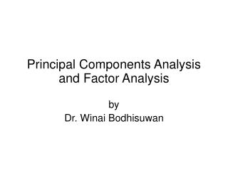
All principal components (PCs) start at the origin of the ordinate axes. First PC is direction of maximum variance from origin Subsequent PCs are orthogonal to 1st PC and describe maximum residual variance Principal Components 30 25 20 Wavelength 2 PC 1 15 10 5 0 0 5 10 15 20 25 30 Wavelength 1 30 25 20 PC 2 Wavelength 2 15 10 5 0 0 5 10 15 20 25 30 Wavelength 1
Algebraic Interpretation • Given m points in a n dimensional space, for large n, how does one project on to a low dimensional space while preserving broad trends in the data and allowing it to be visualized?
Algebraic Interpretation – 1D • Given m points in a n dimensional space, for large n, how does one project on to a 1 dimensional space? • Choose a line that fits the data so the points are spread out well along the line
Algebraic Interpretation – 1D • Formally, minimize sum of squares of distances to the line. • Why sum of squares? Because it allows fast minimization, assuming the line passes through 0
Algebraic Interpretation – 1D • Minimizing sum of squares of distances to the line is the same as maximizing the sum of squares of the projections on that line, thanks to Pythagoras.
Algebraic Interpretation – 1D • How is the sum of squares of projection lengths expressed in algebraic terms? L i n e P P P … P t t t … t 1 2 3 … m Point 1 Point 2 Point 3 : Point m L i n e xT BT B x
PCA: General From k original variables: x1,x2,...,xk: Produce k new variables: y1,y2,...,yk: y1 = a11x1 + a12x2 + ... + a1kxk y2 = a21x1 + a22x2 + ... + a2kxk ... yk = ak1x1 + ak2x2 + ... + akkxk
PCA: General From k original variables: x1,x2,...,xk: Produce k new variables: y1,y2,...,yk: y1 = a11x1 + a12x2 + ... + a1kxk y2 = a21x1 + a22x2 + ... + a2kxk ... yk = ak1x1 + ak2x2 + ... + akkxk such that: yk's are uncorrelated (orthogonal) y1 explains as much as possible of original variance in data set y2 explains as much as possible of remaining variance etc.
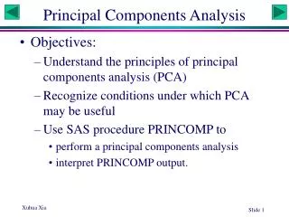
2nd Principal Component, y2 1st Principal Component, y1
xi2 yi,1 yi,2 xi1 PCA Scores
λ2 λ1 PCA Eigenvalues
PCA: Another Explanation From k original variables: x1,x2,...,xk: Produce k new variables: y1,y2,...,yk: y1 = a11x1 + a12x2 + ... + a1kxk y2 = a21x1 + a22x2 + ... + a2kxk ... yk = ak1x1 + ak2x2 + ... + akkxk yk's are Principal Components such that: yk's are uncorrelated (orthogonal) y1 explains as much as possible of original variance in data set y2 explains as much as possible of remaining variance etc.
PCA: General {a11,a12,...,a1k} is 1st Eigenvector of correlation/covariance matrix, and coefficients of first principal component {a21,a22,...,a2k} is 2nd Eigenvector of correlation/covariance matrix, and coefficients of 2nd principal component … {ak1,ak2,...,akk} is kth Eigenvector of correlation/covariance matrix, and coefficients of kth principal component
PCA Summary until now • Rotates multivariate dataset into a new configuration which is easier to interpret • Purposes • simplify data • look at relationships between variables • look at patterns of units
PCA Example –STEP 1 • Subtract the mean from each of the data dimensions. All the x values have x subtracted and y values have y subtracted from them. This produces a data set whose mean is zero. Subtracting the mean makes variance and covariance calculation easier by simplifying their equations. The variance and co-variance values are not affected by the mean value.
PCA Example –STEP 1 DATA: x y 2.5 2.4 0.5 0.7 2.2 2.9 1.9 2.2 3.1 3.0 2.3 2.7 2 1.6 1 1.1 1.5 1.6 1.1 0.9 ZERO MEAN DATA: x y .69 .49 -1.31 -1.21 .39 .99 .09 .29 1.29 1.09 .49 .79 .19 -.31 -.81 -.81 -.31 -.31 -.71 -1.01
PCA Example –STEP 2 • Calculate the covariance matrix cov = .616555556 .615444444 .615444444 .716555556 • since the non-diagonal elements in this covariance matrix are positive, we should expect that both the x and y variable increase together.
PCA Example –STEP 3 • Calculate the eigenvectors and eigenvalues of the covariance matrix eigenvalues = .0490833989 1.28402771 eigenvectors = -.735178656 -.677873399 .677873399 -.735178656
PCA Example –STEP 3 • eigenvectors are plotted as diagonal dotted lines on the plot. • Note they are perpendicular to each other. • Note one of the eigenvectors goes through the middle of the points, like drawing a line of best fit. • The second eigenvector gives us the other, less important, pattern in the data, that all the points follow the main line, but are off to the side of the main line by some amount.
PCA Example –STEP 4 • Reduce dimensionality and form feature vector the eigenvector with the highest eigenvalue is the principle component of the data set. In our example, the eigenvector with the larges eigenvalue was the one that pointed down the middle of the data. Once eigenvectors are found from the covariance matrix, the next step is to order them by eigenvalue, highest to lowest. This gives you the components in order of significance.
PCA Example –STEP 4 Now, if you like, you can decide to ignore the components of lesser significance. You do lose some information, but if the eigenvalues are small, you don’t lose much • n dimensions in your data • calculate n eigenvectors and eigenvalues • choose only the first p eigenvectors • final data set has only p dimensions.
PCA Example –STEP 4 • Feature Vector FeatureVector = (eig1 eig2 eig3 … eign) We can either form a feature vector with both of the eigenvectors: -.677873399 -.735178656 -.735178656 .677873399 or, we can choose to leave out the smaller, less significant component and only have a single column: - .677873399 - .735178656
Reconstruction of original Data x -.827970186 1.77758033 -.992197494 -.274210416 -1.67580142 -.912949103 .0991094375 1.14457216 .438046137 1.22382056