Aquarius Algorithm Workshop: Simulation Studies and Calibration Strategies
The Aquarius Algorithm Workshop, held from March 9-11, 2010, in Santa Rosa, CA, focused on simulation studies crucial for the calibration and analysis of the Aquarius instrument. Led by Principal Investigator Gary Lagerloef, the workshop covered several key aspects including crossover analysis, AVDS matchups, and methods for managing on-orbit anomalies. Attendees developed tools for de-biasing approaches and explored potential scenarios involving arbitrary biases across all channels. The workshop aimed at establishing a solid foundation for the commissioning phase leading up to the orbital readiness review (ORR).

Aquarius Algorithm Workshop: Simulation Studies and Calibration Strategies
E N D
Presentation Transcript
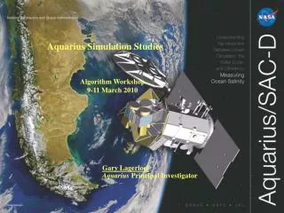
Aquarius Simulation Studies Algorithm Workshop 9-11 March 2010 Gary Lagerloef Aquarius Principal Investigator
Outline • IOC phase preparation • Crossover analysis • AVDS matchups & other de-bias approaches • On-orbit anomalies and calibration drifts • Potential scenarios (i.e. with noise/error) • Insert arbitrary biases in all 12 channels • Timetable between now and ORR (Sep 2010)
Aquarius Instrument Commissioning Timeline L+25 L+26 L+27 L+28 L+30 L+32 L+34 L+35 L+29 L+31 L+33 Time from launch (days) 11 days L+45 2 3 4 5 6 7 8 9 10 1 AQ Instrument Deployment & Checkout Phase Mission Phase SAC-D instruments on Upload patches AQ Activities Verify S/P config ICDS ON ICDS ATC On ATC Config ATC cntrlr Deply Boom Deply reflector Antenna Deployment Deply heaters on DPU off DPU On DPU + RFEs + RBEs ON DPU On Radiometer SCAT Rx only SCAT Tx single beam SCAT Tx ALL beam Scatterometer Instrument preliminary Performance assessment Post Launch Assessment Review PLAR Ground Coverage NEN Cordoba Matera Mission Design Team Product
Remove orbit errors Continue algorithm development and test with new simulator data Beam 1 SSS (with harmonic errors added) Beam 2 SSS (with constant and harmonic errors added) Adjusted Beam 1 SSS (with harmonic errors removed) Adjusted Beam 2 SSS (with constant and harmonic errors removed)
Science Implementation Milestones • 1 March 2010: Science simulator – CY2007 Level 2 (swath) and Level 3 (gridded map) files released • 9-11 March 2010: Aquarius algorithm science team workshop, Santa Rosa, CA • 30 March 2010 until Launch: • Operational simulator generates daily files, • Analysis and evaluation by science team • 1 April – to – ORR: (September) • Science team develops and tests Aquarius commissioning phase analysis tools. • Use simulators and tools to develop and test case studies, anomalies and rehearsals. • 19-21 July 2010: Aquarius/SAC-D Science Team meeting, Seattle • ORR: Final commissioning phase plan; analysis tools tested and ready.
Search Radius Buoy Obs. Approaches to De-biasing • Each radiometer needs to be independently calibrated • First try to remove the gross offsets in the initial retrieved SSS • Use reference salinity field globally • AVDS matchups – tabulate for each beam • Cross-over analysis to remove residual inter-beam biases • With time, work through the re-calibration of retrieval coefficients • Match-up processing • One match-up file per buoy observation contains all the satellite data in the search radius • Subsequent processing to generate the optimal weighted average satellite observation per buoy • Global tabulations
Potential scenarios / rehearsals Simulate certain special situations to test and analyze Develop and test analysis tools Demonstrate we can address these issues at ORR • Insert arbitrary biases in all 12 channels • Simulate arbitrary drifts in all 12 channels • Orbit harmonics calibration drifts (1-4 harmonics, e.g.) • Simulate a complete cold sky maneuver • Solar flare • RFI • Attitude offsets • Channel failure • H or V channel • P or M channel • Other suggestions … lunar, bi-static solar reflection, diffuse galaxy refl.
Approach • Generate a set of special case 7-day cycles • Specify cases: biases, drifts, etc • Decide who generates them? ADPS or RSS? • Generate these scenarios with either the 2007 simulator or the operational simulator. • Timetable: • 30 May: Produce scenarios (L2 files) • June-July: Analysis; preliminary results at July Science meeting • August: Assess results (special workshop?) • September: ORR
Other issues • Filename convention: add cycle/orbit numbers ? • 103 orbits per cycle • When to start cycle #1? • Alternative retrievals • 1st Stokes only • H or V only • Use Tp and Tm • Different algorithms for different beams depending on specific channel behavior.
Back-up Slides with detail activities for each commissioning phase Science Task
Science Task 1 • Task: Generate simulated data for radiometer (TA) and scatterometer (sigma0); • Simulation reflects actual orbit and spacecraft attitude; • 7-10 days of data simulated; • Prepared 5 days prior to instrument turn-on (for use by engineering team) and updated as necessary. • Available to engineering team on location at MOC. • Objectives: • Engineering: Simulated TA and sigma0 for the engineering team to use during on-orbit check out to judge reasonableness of the actual measured signals; • Science: A reference signal for use by science team to begin evaluation of the science quality of the first signals. • Representative Roles and Responsibilities: • Wentz: Radiometer TA simulations; • Yueh: Scatterometer Sigma0 simulations.
Science Task 2 • Task: Examine radiometer data to judge whether or not the radiometer data is reasonable • Begins on day 4 after radiometer is completely turned on; • Continues through end of commissioning (PLAR); • Initially, thermal stability may not be ideal. • Objectives: • Collect reference data prior to the turn on of other instruments (Scat and CONAE) as baseline to judge interference; • Collect data to assess acceptance criteria for PLAR; • Representative Roles and Responsibilities: • Wentz: Examine TA to asses pointing accuracy; • Le Vine: Evaluate T3 and retrieved Faraday rotation; • Ruf: Evaluate RFI environment and detection algorithm; • Brown: Compare histograms of actual and model TB; • Lagerloef: Start processing AVDS matchups.
Science Tasks 3 - 5 • Task: Examine scatterometer data during turn on of the instrument • Days 5-7 during 3-day turn-on sequence for the scatterometer; • Radiometer is on and collecting data. • Objectives: • Examine radiometer data for evidence of scatterometer interference (engineering team will also be looking at raw data); • Examine scatterometer data for reasonable behavior. • Representative Roles and Responsibilities • Yueh and scatterometer engineering team: Examine loopback power, noise only measurements and echo power; • Yueh: Analyze correlation of sigma0 with winds (NCEP). • Radiometer team (Wentz, Le Vine, Brown, others): Examine radiometer data before and after scatterometer turn-on for evidence of interference.
Science Task 6 • Task: Examine Aquarius instrument data (scatterometer and radiometer) for nominal behavior • Days 8-10 after both instruments are turned on completely; • First nominal operation; • Objectives: • Continue with radiometer science data evaluation begun in Task 2; • Begin evaluation of scatterometer data in nominal mode; • First look at instrument stability; • Comparison of data at reference sites and at cross-over points. • Representative Roles and Responsibilities • Ruf: Collect data for first look at “vicarious” calibration; • Le Vine: Compare Faraday rotation retrieved from T3 with in situ (ground sounders) truth; • Wentz: Pointing accuracy and effect of Sun; • Yueh: First look at roughness correction for radiometer.
Science Task 7 • Task: Nominal Aquarius instrument operation (radiometer and scatterometer) and CONAE instrument turn on; • Day 11 - TBD: Nominal Aquarius operation • CONAE instruments start turn on. • Science team activities continue from previous tasks. • Objectives: • Examine radiometer data for evidence of interference from CONAE instruments; • Generate first 7-day global map of SSS • Continue to collect data to assess acceptance criteria for PLAR. • Representative Roles and Responsibilities • Science Team: Coordinate data collection with CONAE instrument turn-on to search for evidence of interference; • Lagerloef: Generate reference SSS map from Argo data and de-bias Aquarius SSS output; • Yueh: Roughness correction and correlation of sigma0 with NCEP and other sources of data on winds.
We will begin processing AVDS matchups as soon as the radiometer subsystem is turned on, including the warm-up transients. • Use in situ SSS and SST to estimate expected TAs for comparison to observed TAs, as well as comparing derived SSS. • Examine trends in observed vs expected TA difference vs wind speed. • We will compute cross-over differences between ascending and descending passes to: • Monitor the drifts and offsets of channels relative to each other • Look for solar interference signature • Examine consistency to TA differences for various channels vs incidence angle difference and pointing accuracy • Detect and remove retrieved SSS biases between channels and produce a preliminary composite SSS map. • Data Requirements: L2 science data file immediately after processing • Tools: • AVDS-ADPS matchup processing is mature – will continue testing with operational simulator. • AVDS matchup processing tools are being written – designed to tabulate satellite-in situ differences and ancillary data. • Analysis tools will be developed in an evolutionary process as we work with matchups with the operational simulator.
Science Commissioning Approach • Post-launch in-orbit checkout simulation: During the period from launch to L+25 days, the science team will compute simulated Tb and σ0 based on the final orbit after maneuvers (Science Task 1) • These data will provide “Expected Values” for each beam along-track to compare quantitatively with observations for both the engineering and science acceptance analyses • The science team will carry out an analysis sequence (Science Tasks 2-7) at each stage of the instrument turn-on sequence • Acceptance criteria are limited: • The timeline only allows for one 7-day cycle after the instrument is fully turned on • Assess whether the data are “as expected” in qualitative terms and the sensor is “calibrate-able” • Gross geographical and geophysical features are as expected, biases can be removed, stability is reasonable, polarization differences are appropriate, etc. (details below)
Preliminary Acceptance Criteria • Engineering Evaluation of the Instrument Complete • Internal checks are complete and nominal (temperature, voltage, currents, telemetry) • Instrument L3 requirements are met • Antenna deployment is nominal • Thermal control system nominal • Radiometer Specific Criteria • Radiometer internal performance nominal (consistent with observations pre-launch) • Gain, NEDT, Counts Level, Noise Diode Ratios • Radiometer gain stability nominal at the operational thermal set point • Antenna Pointing Verified (scenes and transitions where expected) • Interference from Scatterometer or other SAC-D instruments within specifications • Predictable Science Response (consistent with simulations) • Land - ocean features evident in radiometer brightness temperature (Tb) both in contrast and location; • Relative polarization levels (V compared to H) for each beam are consistent with the emissivity model; • Relative levels of Tb among beams is consistent with emissivity model (e.g. V-pol signal increasing and H-pol decreasing with increased incidence angle); • The 3rd Stokes signal consistent with expectation (small signal varying with Faraday rotation); • Reasonable initial “first-look” 7-day salinity map consistent with climatology • Scatterometer Specific Criteria • Receiver gain and receiver noise within expected range • Transmit power-receive gain product (loopback) within expected range • Losses of cables between RFE and OMT are stable (inferred from CND; applies to radiometer) • Antenna pointing stable (land-water signals as expected and repeatable) • σ0 of ocean and land within expected range for each beam.