Handwritten digit recognition
Handwritten digit recognition. Jitendra Malik. Handwritten digit recognition (MNIST,USPS). LeCun’s Convolutional Neural Networks variations (0.8%, 0.6% and 0.4% on MNIST) Tangent Distance( Simard , LeCun & Denker : 2.5% on USPS)


Handwritten digit recognition
E N D
Presentation Transcript
Handwritten digit recognition Jitendra Malik
Handwritten digit recognition (MNIST,USPS) • LeCun’s Convolutional Neural Networks variations (0.8%, 0.6% and 0.4% on MNIST) • Tangent Distance(Simard, LeCun & Denker: 2.5% on USPS) • Randomized Decision Trees (Amit, Geman & Wilder, 0.8%) • K-NN based Shape context/TPS matching (Belongie, Malik & Puzicha: 0.6% on MNIST) • SVM on orientation histograms(Maji & Malik, 0.8%)
The MNIST DATABASE of handwritten digitsyann.lecun.com/exdb/mnist/YannLeCun & Corinna Cortes • Has a training set of 60 K examples (6K examples for each digit), and a test set of 10K examples. • Each digit is a 28 x 28 pixel grey level image. The digit itself occupies the central 20 x 20 pixels, and the center of mass lies at the center of the box. • “It is a good database for people who want to try learning techniques and pattern recognition methods on real-world data while spending minimal efforts on preprocessing and formatting.”
The machine learning approach to object recognition • Training time • Compute feature vectors for positive and negative examples of image patches • Train a classifier • Test Time • Compute feature vector on image patch • Evaluate classifier
In feature space, positive and negative examples are just points…
Different approaches to training classifiers • Nearest neighbor methods • Neural networks • Support vector machines • Randomized decision trees • …
Linear Separators (aka. Perceptrons) Support Vector Machines
Other possible solutions Support Vector Machines
Which one is better? B1 or B2? How do you define better? Support Vector Machines
Find hyperplane maximizes the margin => B1 is better than B2 Support Vector Machines
Support Vector Machines Examples are; (x1,..,xn,y) with y{-1.1}
Some remarks.. • While the diagram corresponds to a linearly separable case, the idea can be generalized to a “soft margin SVM” where mistakes are allowed but penalized. • Training an SVM is a convex optimization problem, so we are guaranteed that we can find the globally best solution. Various software packages are available such as LIBSVM, LIBLINEAR • But what if the decision boundary is horribly non-linear? We use the “kernel trick”
We can construct a new higher-dimensional feature space where the boundary is linear
Kernel Support Vector Machines • Kernel : • Inner Product in Hilbert Space • Can Learn Non Linear Boundaries
linear SVM, KernelizedSVM Decision function is where: Linear: Non-linear Using Kernel
Transformation invariance(or, why we love orientation histograms so much!) • We want to recognize objects in spite of various transformations-scaling, translation, rotations, small deformations… of course, sometimes we don’t want full invariance – a 6 vs. a 9
How do we build in transformational invariance? • Augment the dataset • Include in it various transformed copies of the digit, and hope that the classifier will figure out a decision boundary that works • Build in invariance into the feature vector • Orientation histograms do this for several common transformations and this is why they are so popular for building feature vectors in computer vision • Build in invariance into the classification strategy • Multi-scale scanning deals with scaling and translation
Orientation histograms • Orientation histograms can be computed on blocks of pixels, so we can obtain tolerance to small shifts of a part of the object. • For gray-scale images of 3d objects, the process of computing orientations, gives partial invariance to illumination changes. • Small deformations when the orientation of a part changes only by a little causes no change in the histogram, because we bin orientations
Some more intuition • The information retrieval community had invented the “bag of words” model for text documents where we ignore the order of words and just consider their counts. It turns out that this is quite an effective feature vector – medical documents will use quite different words from real estate documents. • An example with letters: How many different words can you think of that contain a, b, e, l, t? • Throwing away the spatial arrangement in the process of constructing an orientation histogram loses some information, but not that much. • In addition, we can construct orientation histograms at different scales- the whole object, the object divided into quadrants, the object divided into even smaller blocks.
We compare histograms using the Intersection Kernel Histogram Intersection kernel between histograms a, b K small -> a, b are different K large -> a, b are similar Intro. by Swain and Ballard 1991 to compare color histograms. Odone et al 2005 proved positive definiteness. Can be used directly as a kernel for an SVM.
What is the Intersection Kernel? Histogram Intersection kernel between histograms a, b
What is the Intersection Kernel? Histogram Intersection kernel between histograms a, b K small -> a, b are different K large -> a, b are similar Intro. by Swain and Ballard 1991 to compare color histograms. Odone et al 2005 proved positive definiteness. Can be used directly as a kernel for an SVM. Compare to
Digit Recognition using SVMS Jitendra Malik Lecture is based on Maji & Malik (2009)
Digit recognition using SVMs • What feature vectors should we use? • Pixel brightness values • Orientation histograms • What kernel should we use for the SVM? • Linear • Intersection kernel • Polynomial • Gaussian Radial Basis Function
Some popular kernels in computer visionx and y are two feature vectors
Kernelized SVMs slow to evaluate Decision function is where: Sum over all support vectors Kernel Evaluation Feature vector to evaluate Feature corresponding to a support vector l Arbitrary Kernel Histogram Intersection Kernel Cost:# Support Vectors x Cost of kernel computation
Complexity considerations • Linear kernels are the fastest • Intersection kernels are nearly as fast, using the “Fast Intersection Kernel” (Maji, Berg & Malik, 2008) • Non-linear kernels such as the polynomial kernel or Gaussian radial basis functions are the slowest, because of the need to evaluate kernel products with each support vector. There could be thousands of support vectors!
Raw pixels do not make a good feature vector • Each digit in the MNIST DATABASE of handwritten digits is a 28 x 28 pixel grey level image.
Some key references on orientation histograms • D. Lowe, ICCV 1999, SIFT • A. Oliva & A. Torralba, IJCV 2001, GIST • A. Berg & J. Malik, CVPR 2001, Geometric Blur • N. Dalal & B. Triggs, CVPR 2005, HOG • S. Lazebnik, C. Schmid & J. Ponce, CVPR 2006, Spatial Pyramid Matching
Kernelized SVMs slow to evaluate Decision function is where: Sum over all support vectors Kernel Evaluation Feature vector to evaluate Feature corresponding to a support vector l Arbitrary Kernel Histogram Intersection Kernel SVM with Kernel Cost: # Support Vectors x Cost of kernel comp. IKSVM Cost: # Support Vectors x # feature dimensions
Randomized decision trees(a.k.a. Random Forests) Jitendra Malik
Two papers • Y. Amit, D. Geman & K. Wilder, Joint induction of shape features and tree classifiers, IEEE Trans. on PAMI, Nov. 1997.(digit classification) • J. Shotton et al, Real-time Human Pose Recognition in Parts from Single Depth Images, IEEE CVPR, 2011. (describes the algorithm used in the Kinect system)
Decision trees for Classification • Training time • Construct the tree, i.e. pick the questions at each node of the tree. Typically done so as to make each of the child nodes “purer”(lower entropy). Each leaf node will be associated with a set of training examples • Test time • Evaluate the tree by sequentially evaluating questions, starting from the root node. Once a particular leaf node is reached, we predict the class to be the one with the most examples(from training set)at this node.
Amit, Geman & Wilder’s approach • Some questions are based on whether certain “tags” are found in the image. Crudely, think of these as edges of particular orientation. • Other questions are based on spatial relationships between pairs of tags. An example might be whether a vertical edge is found above and to the right of an horizontal edge