Matched Filtering as a Tool for Separating Magnetic Signal Sources
This article examines matched filtering as a method to distinguish between shallow and deep source layers in total magnetic intensity maps. Using a Fourier transform approach, model parameters derived from the power spectrum are employed to design optimal filters for signal separation. The statistical model involves vertical-sided prisms and focuses on the depth term, while ignoring size and thickness for simplicity. By analyzing amplitude and wavenumber, we derive parameters necessary for filtering. The graphical representation highlights the effectiveness of the matched filters for both layers.

Matched Filtering as a Tool for Separating Magnetic Signal Sources
E N D
Presentation Transcript
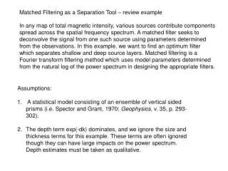
Matched Filtering as a Separation Tool – review example In any map of total magnetic intensity, various sources contribute components spread across the spatial frequency spectrum. A matched filter seeks to deconvolve the signal from one such source using parameters determined from the observations. In this example, we want to find an optimum filter which separates shallow and deep source layers. Matched filtering is a Fourier transform filtering method which uses model parameters determined from the natural log of the power spectrum in designing the appropriate filters. • Assumptions: • A statistical model consisting of an ensemble of vertical sided prisms (i.e. Spector and Grant, 1970; Geophysics, v. 35, p. 293-302). • The depth term exp(-dk) dominates, and we ignore the size and thickness terms for this example. These terms are often ignored though they can have large impacts on the power spectrum. Depth estimates must be taken as qualitative.
Plot ln(amplitude2) vs wavenumber • Pick deep linear segment • Find the slope slope = (6 - -6) / 0.60 = -20 depth = D = -slope/2 = 10 • Find C intercept ~ 5.8 ln (C2) = 5.8 C = sqrt(exp(5.8)) = 18 • Do the same for the shallow layer • depth = d = 2 c = 1 We now have the parameters (c, C, d, D) for the matched filter to separate the regional, deep layer:
Graphing the matched filter: yields the magenta line and yields the green line, the matched filter for the shallow layer. Multiplying (in 2D) these times the Fourier transform of the total magnetic field separates the layers subject to all assumptions.