Download
1 / 47
490 likes | 646 Vues
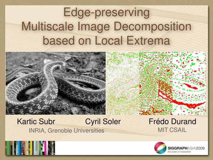
Edge-preserving Multiscale Image Decomposition based on Local Extrema. Kartic Subr Cyril Soler Frédo Durand. MIT CSAIL. INRIA, Grenoble Universities. Multiscale image decomposition. 1D. Intensity. Input. Fine. +. Medium. +. Coarse. Pixels. Motivation.

E N D
Edge-preserving Multiscale Image Decomposition based on Local Extrema Kartic Subr Cyril Soler Frédo Durand MIT CSAIL INRIA, Grenoble Universities
Multiscale image decomposition 1D Intensity Input Fine + Medium + Coarse Pixels
Motivation Detail enhancement Separating fine texture from coarse shading
Related work Linear multiscale methods Edge-preserving approaches 1D Signal analysis
Related work: Linear multiscale methods Edge-preserving approaches [Lindeberg 94] [Burt and Adelson 93] Edges not preserved 1D Signal analysis (Causes halos while editing) [Rahman and Woodell 97] [Pattanaik et al 98]
Related work: Edge-preserving methods [Fattal et al 07] [Farbman et al 08] Edge-aware Assume detail is low contrast 1D Signal analysis [Chen et al 07] [Bae et al 07]
Related work: Empirical mode decomposition Linear multiscale Edge-preserving approaches [Huang et al 98] Developed for 1D signals Detail depends on spatial scale Not edge-aware
Existing edge-preserving image decompositions Edge (preserved) Input Detail (smoothed) Assume detail is low-intensity variation Edge-preserving smoothing (e.g. bilateral filter) Base layer + Detail layer (Input – Base)
Challenge: Smoothing high-contrast detail High-contrast detail Edge Low-contrast detail
Challenge: Smoothing high-contrast detail High-contrast detail smoothed? Edge preserved? Low-contrast detail smoothed? Conservative smoothing (bilateral filter with narrow range-Gaussian)
Challenge: Smoothing high-contrast detail High-contrast detail smoothed? Edge preserved? Low-contrast detail smoothed? Aggressive smoothing (bilateral filter with wide range-Gaussian)
Example: Smoothing high-contrast detail Detail not smoothed Detail not smoothed Edge smoothed Coarse features smoothed Input [Farbman et al 2008] λ= 13, α= 0.2 [Farbman et al 2008] λ= 13, α= 1.2
Our approach: Use local extrema Detail = oscillations between local extrema Local maxima Input Local minima
Our approach: Use local extrema Base = Local mean of neighboring extrema
Our approach: Use local extrema High-contrast detail smoothed? Edge preserved? Low-contrast detail smoothed? Local mean of neighboring extrema
Our detail extraction Input High-contrast detail smoothed Base layer + Edges preserved Detail layer
Algorithm Input: Image + number of layers Identify local extrema Estimate smoothed mean Detail at multiple scales
Algorithm: Identifying local extrema Extrema detection kernel Local maxima Local minima
Algorithm: Estimating smoothed mean 1) Construct envelopes Maximal envelope Minimal envelope Interpolation preserves edge [Levin et al 04]
Algorithm: Estimating smoothed mean 2) Average envelopes Estimated mean
Algorithm: After one iteration Input Base + Detail
Algorithm: Mean at coarser scale Widen extrema detection kernel Local maxima Local minima
Algorithm: Mean at coarser scale Maximal envelope Minimal envelope
Algorithm: Mean at coarser scale Estimated mean
Recap: Detail extraction Input Identify local extrema Construct envelopes Base Detail = Input - Base Average envelopes Smoothed mean
Recap: Multiscale decomposition Iteration 1 on input Layer 3 Layer 2 Layer 1 Input Coarse Fine Iteration 2 on B1 Base B1 Detail D1 Recurse n-1 times for n-layers Detail D2 Base B2
Results: Smoothing Input Smoothed
Results: Multiscale decomposition Input Low contrast edge Low contrast edge High contrast detail High contrast detail Coarse Medium Fine
Results: Multiscale decomposition Fine Coarse
Comparison Our Result [Farbman et al 2008]
Limitation Input Our Result
Conclusion Detail based on local extrema Smoothing high contrast detail Edge-preserving multiscale decomposition
Acknowledgements INRIA post-doctoral fellowship HFIBMR grant(ANR-07-BLAN-0331) Equipe Associée withMIT ‘Flexible Rendering’ Adrien Bousseau & Alexandrina Orzan Anonymous reviewers