Efficient Distinct Letter Detection in Images using Breadth-First Search (BFS)
This document outlines an application that utilizes the Breadth-First Search (BFS) algorithm with a queue to identify distinct letters in an image. By scanning the image row by row and connecting white pixels, the algorithm counts distinct symbols and draws bounding boxes around them. The process involves maintaining coordinates that define the bounding box for each connected group of white pixels. This method enhances accuracy in detecting and visualizing characters, providing a robust solution for image analysis.

Efficient Distinct Letter Detection in Images using Breadth-First Search (BFS)
E N D
Presentation Transcript
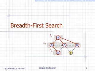
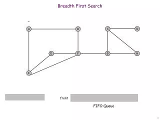
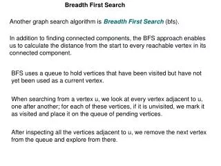
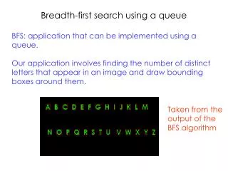
Breadth-first search using a queue BFS: application that can be implemented using a queue. Our application involves finding the number of distinct letters that appear in an image and draw bounding boxes around them. Taken from the output of the BFS algorithm
Overall idea behind the algorithm Scan the pixels of the image row by row, skipping over black pixels until you encounter a white pixel p(j,k). (j and k are the row and column numbers of this pixel.) Now the algorithm uses a queue Q to identify all the white pixels that are connected together with p(j,k) to form a single symbol/character in the image. When the queue becomes empty, we would have identified all the pixels that form this character (and assigned the color Green to them.) While identifying these connected pixels, also maintain the four variables lowx, highx, lowy and highy. These are the bounding values. When the queue is empty, these bounding values are the x- and y-coordinates of the bounding box.
Let the image width be w and the height be h; Set visited[j,k] = false for all j,k; count = 0; Initialize Q; // count is the number of symbols in the image. for j from 1 to w – 1 do for k from 0 to h – 1 do if (color[j,k] is white) then count++; lowx = j; lowy = k; highx = j; highy = k; insert( [j,k]) into Q; visited[j,k] = true; while (Q is not empty) do p = delete(Q); let p = [x,y];color[x,y] = green; if x < lowx then lowx = x;if y < lowy then lowy = y; if x > highx then highx = x;if y > highy then highy = y; for each neighbor n of p do if visited[n] is not true then visited[n] = true; if (color[n] is white) insert(n) into Q; end if; end if; end for; end while; draw a box with (lowx-1,lowy-1) as NW and (highx + 1, highy + 1) as SE boundary; // make sure that highx+1 or highy+1 don’t exceed the dimensions else visited[j,k] = true;end if; end do; end do;
Example: 0 1 2 3 4 5 6 7 0 1 2 3 4 5 6 7
Example: when the algorithm stops, count would be 1 xlow = 2 xhigh = 6 ylow = 1 yhigh = 7 Draw the bounding box (2,1), (2,6), (7,1) and (7, 6). 0 1 2 3 4 5 6 7 0 1 2 3 4 5 6 7
Example: when the algorithm stops, count would be 1 xlow = 2 xhigh = 6 ylow = 2 yhigh = 7 Draw the bounding box (2,1), (2,6), (7,1) and (7, 6). 0 1 2 3 4 5 6 7 0 1 2 3 4 5 6 7
Example: 0 1 2 3 4 5 6 7 count = 0 Q = { } visited changes as shown in fig. 0 1 2 3 4 5 6 7 t t
Example: 0 1 2 3 4 5 6 7 count = 1; lowx = highx = 2 lowy = highy = 3 Q = {(2,3)} 0 1 2 3 4 5 6 7 t t t
Example: 0 1 2 3 4 5 6 7 0 1 2 3 4 5 6 7 After first Q.delete(): Q = { } count = 1; lowx = highx = 2 lowy = highy = 3 Q = {(3, 3)} t t t t
Example: 0 1 2 3 4 5 6 7 After second Q.delete(): Q = { } P = (3,3) color[p] = green lowx = 2 highx = 3 lowy = highy = 3 Q = {(4,3), (3,4)} 0 1 2 3 4 5 6 7 t t t t t t
Example: 0 1 2 3 4 5 6 7 After third delete(Q): Q = {(3,4)} P = (4,3) color[p] = green lowx = 2 highx = 4 lowy = highy = 3 Q = {(3,4),(5,3)} 0 1 2 3 4 5 6 7 t t t t t t t
Example: After fourth delete(Q): visited[3,4]= true Q = {(5, 3)} P = (3, 4) color[p] = green lowx = 2 highx = 4 lowy = 3 highy = 4 Q = {(5,3),(3,5)} 0 1 2 3 4 5 6 7 0 1 2 3 4 5 6 7 t t t t t t t t
Example: After fifth delete(Q): visited[5,3]= true Q = {(3,5)} P = (3, 5) color[p] = green lowx = 2 highx = 5 lowy = 3 highy = 4 Q = {(3,5)} 0 1 2 3 4 5 6 7 0 1 2 3 4 5 6 7 t t t t t t t t
Example: After sixth delete(Q): visited[5, 3]= true Q = {} P = (5, 3) color[p] = green lowx = 2 highx = 5 lowy = 3 highy = 5 Q = {(3,6)} 0 1 2 3 4 5 6 7 0 1 2 3 4 5 6 7 t t t t t t t t
Example: After seventh delete(Q): visited[3,6]= true Q = { } P = (3,6) color[p] = green lowx = 2 highx = 5 lowy = 3 highy = 6 Q = {(3,7)} 0 1 2 3 4 5 6 7 0 1 2 3 4 5 6 7 t t t t t t t t t
Example: After eighth delete(Q): visited[3,7]= true Q = { } P = (3,7) color[p] = green lowx = 2 highx = 5 lowy = 3 highy = 7 Q = { } At this point the while loop ends. 0 1 2 3 4 5 6 7 0 1 2 3 4 5 6 7 t t t t t t t t t