Alon Arad
Hurst Exponent of Complex Networks. Alon Arad. Outline. Introduction Random Graph Types of Network Models Studied The Hurst Exponent Linear Algebra and the Adjacent Matrix Results and Conclusion. Introduction.

Alon Arad
E N D
Presentation Transcript
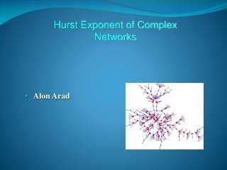
Hurst Exponent of Complex Networks Alon Arad
Outline Introduction Random Graph Types of Network Models Studied The Hurst Exponent Linear Algebra and the Adjacent Matrix Results and Conclusion
Introduction Used Rescaled Range Analysis and the adjacency matrix to study the spacing between eigenvalues for three widely used network models
The Random Graph Initially proposed to model complex networks Had well defined properties. Properties of Random processes have been widely studied Model was not small enough Clustering Co-efficient was not correct.
The Three Models Poisson random graph of Erdos and Renyi Ensemble of all graphs having V vertices E edges Each pair of vertices connected with probability P Clearly Graph model needed to be improved
The Three Models Small world model of Watts and Strogatz Example widely used is the one dimensional example A ring with V vertices Each vertex joined to another k lattice spacing away Vk edges Now take edge, with probability P, move to another point in lattice chosen at random If P=0 we have regular lattice, if P=1 we have previous model Small world is somewhere in between
The Three Models Preferential attachment of Barbasi and Albert Start with V1 unconnected nodes Attach nodes one at a time to existing node with probability P Probability is biased It is proportional to number of links existing node already has Gives a power law distribution Scale free – will have same properties no matter how many nodes Most resembles a real network system
The Big Question Real Networks Fat tails, power law distributed, scale free Power Law We all know that the power law is synonymous with fractal type behavior Question The question we are all asking ourselves is, how fractals are the graph models described
Rescaled Range (R/S) Analysis Method Rescaled range analysis studies the distribution of events by grouping observed data into clusters of different sizes and studying the scaling behavior of the statistical parameters with the cluster sizes.
In the Beginning In 1951, Hurst defined a method to study natural phenomena such as the flow of the Nile River. Process was not random, but patterned. He defined a constant, K, which measures the bias of the fractional Brownian motion. In 1968 Mandelbrot defined this pattern as fractal. He renamed the constant K to H in honor of Hurst. The Hurst exponent gives a measure of the smoothness of a fractal object where H varies between 0 and 1.
Random and not Random It is useful to distinguish between random and non-random data points. If H equals 0.5, then the data is determined to be random. If the H value is less than 0.5, it represents anti-persistence. If the H value varies between 0.5 and 1, this represents persistence. (what we get)
Calculation of R/S Start with the whole observed data set that covers a total duration and calculate its mean over the whole of the available data
Calculation of R/S Sum the differences from the mean to get the cumulative total at each increment point, V(N,k), from the beginning of the period up to any point, the result is a series which is normalized and has a mean of zero
Calculation of R/S Calculate the range
Calculation of R/S Calculate the standard deviation
Calculation of R/S Plot log-log plot that is fit Linear Regression Y on X where Y=log R/S and X=log n where the exponent H is the slope of the regression line.
The Adjacent Matrix Adjacent matrix characterizes the topology of the network in more usable form A graph is completely determined by its vertex set and by a knowledge of which pairs of vertices are connected Make a graph with m vertices The adjacent matrix is an m×m matrix defined by A = [aij] in which aij =1 if vi is connected to vj, and is 0 otherwise.
We have a problem The matrix of the graph can be contrived in multiple ways depending on how the vertices are labeled. We can show that two unequal matrices in fact represent the same graph.
Solution R/S applied to study the distribution of spacing Not of the actual adjacency matrix But the eigenvalues of adjacency matrix This process will be independent of labeling
Results Performed rescales analysis on the three models and the results are as follows
Results All models show persistent behavior Interesting to note that ER model is also persistent Clearly at the limit (ie very large system) we would get H=.5 for ER model
Conclusion I have performed R/S analysis on three types of widely used complex models. I have found that they all exhibit persistent type behaviour If I had more time and available data, I would have performed R/S on a real network. One such possibility I was investigating is the connectivity of international airports.
References University of Melbourne Department of Mathematics and Statistics Notes for 620-222 Linear and Abstract Algebra Semester 2 2005. Kazumoto Iguchi and Hiroaki Yamada, Exactly solvable scale-free network model, Physical Review E 71, 036144 (2005) O. Shanker, Hurst Exponent of spectra of Complex Networks June 4, 2006 PACS number 89.75.-k. Fractal Maket Analysis, Edgar E. Peters,1994 Introductory Graph Theory, Gary Chartrand 1977 Introductory Graph Theory , Robin J. Wilso1972

