Data Models
Data Models. Based in part on Chapter 2 in Database Systems (Rob and Coronel). Degrees of Separation. In the early 1970’s, the Data Base Task Group (DBTG) identified two levels important to distinguish in database design. The schema is the logical design of the entire database.

Data Models
E N D
Presentation Transcript
Data Models Based in part on Chapter 2 in Database Systems (Rob and Coronel)
Degrees of Separation • In the early 1970’s, the Data Base Task Group (DBTG) identified two levels important to distinguish in database design. • The schema is the logical design of the entire database. • The sub-schema is the logical design of part of the database seen by a particular user or application (a view). • Codd, Rule 6
Schema vs. Instance • A database schema (its design) should be distinguished from a database instance, which also includes the actual data at any given time. • Analogy: Schema is to instance as class (template) is to object (instantiation) • Similarly, the Data Definition Language (DDL) is used to create/modify the schema, while the Data Manipulation Language (DML) is mainly used to modify or retrieve aspects of the instance.
ANSI-SPARC Architecture • In the mid-1970’s, American National Standards Institute (ANSI) put together the Standards Planning and Requirements Committee (SPARC). • ANSI-SPARC identified three levels important to distinguish in database design. • External • Conceptual • Internal
ANSI-SPARC View 3 View 2 External level View 1 Conceptual Schema Conceptual level Internal Schema Internal level Physical data organization Database
ANSI-SPARC levels • External • Views: only what a user needs to see, arranged in a convenient form • Conceptual • Overall logical view of database (entities, attributes, relationships, constraints, etc.) plus some utilities (security, integrity, etc.) • Internal • Specific information about where and how the data is stored. Interfaces with operating system. • (Physical) • The actual stored data.
DBTG ANSI-SPARC • DBTG’s subschema corresponds to ANSI-SPARC’s external level (the views) • Subschema External schema • DBTG’s schema is divided into two levels in the ANSI-SPARC plan • Conceptual schema • Internal schema
Independence • Recall that E.F. Codd’s Rules 8 and 9 called for physical data independence and logical data independence. • Physical: storage changes don’t effect entities, fields, relationships, etc. • Logical: an extra field need not change the views. • ANSI-SPARC levels help provide this independence.
ANSI-SPARC (Fig. 2.3 in book) View 3 View 1 View 2 External level Logical data independence Conceptual Schema Conceptual level Physical data independence Internal level Internal Schema Physical data organization Database
Same idea/Different words • We distinguished between prescriptive and descriptive approaches. Other terms include: • Prescriptive Procedural (3GL) • Step-by-step procedure for proceeding through database record by record • Descriptive Non-Procedural Declarative (4GL) • Indicate what you want and let the DBMS handle it
4GL Tools • Some of the standard Fourth-generation tools include: • Query generation • Structured Query Language (SQL) • Query By Example (QBE) • Form generation • Report generation
Access Objects 4GL tools in Access: Query, Form, Report and Page generators.
Data Models • A model is “a simplified representation of a system or phenomenon.” (Webster’s) • A data model is a representation of the information associated with an organization. • When we talk about data models, we usually mean an overall approach to representing data (defining it, manipulating it, etc.) rather than some specific representation of some specific organization.
Models and levels • The data models to some extent reflect the level (e.g. prescriptive vs. descriptive) that one operates on. • The older data models (the hierarchical and network models) are based more in a procedural approach. • Whereas the newer relational model is somewhat more declarative. • Even further from implementation details are the Entity-Relationship and Object-Oriented models.
Database History: Hierarchical Model • One of the earliest database models is the Hierarchical Model. • E.g. GUAM and IMS • It is so-called because its logical structure is hierarchical or tree-like. • All relationships in the Hierarchical Model are of the parent-child type. • This is asexual reproduction, a child has one and only one parent.
Example of Hierarchical Logic: Windows Explorer There are files in folders and folders in other folders.
Hierarchical (Tree-like) Structure My Computer A drive? C drive D drive E drive Courses C240 C220 P201 Web C240wks C220wks
Replace the folder names with points to obtain a graph This kind of graph is called a tree. It has no loops.
Problem: what if a file could belong to more than one folder? • A file for CSC 240 may appear on the web page. Does in belong in the C240 folder or the Web\c240wks folder? • To realize both relationships (belonging to CSC 240 and being on the web page) in the Hierarchical Model, one must have two copies of the file. • This would be data redundancy. And if one edits one of the files, we could end up with an “update anomaly.”
Drilling down • Another feature of the hierarchical approach is that it requires “drilling down” (tracing through the entire hierarchy) to get at the data • In the Windows Explorer example, the path requires all of the folders • C:Blum\Courses\C240\TheFile.txt
A note on file systems • The file system (how all of the information is stored on one’s computer) is becoming increasingly database-like. • The current file system typically used with Windows XP NTFS is more like a database than its predecessor FAT32. • In addition Vista and Windows 7 allows the user to opt to have files indexed (for better searching) and also allows the user to add meta tags to file.
Network Model • The Network Model arose in the early 1970s. • The standards for the Network Model were introduced at the Conference on Data Systems Languages (CODASYL) • Example of a Network Model DB: IDS • Its logical structure is a network (a collection of crisscrossing lines). • Unlike the Hierarchical Model, the Network Model’s relationships are not all of the parent-child type.
Example of Network Logic: A Web Site On my web site, I have multiple links to the same set of instructions for making graphs in Excel.
Network Structure La Salle Site My Site Other Faculty Sites My CSC 152 My PHY 105 XY Scatter Plot (Depending on the connections (links), the network approach can lessen the amount of “drilling down” needed.
Replace the web pages with points to obtain a graph This kind of graph is called a network. It has loops. The criss-crossing lines also resemble a web.
Relational Model: History • Introduced by E. F. Codd (early 1970’s). • Was an important step toward the goal of data independence, acting on the higher level, and all that good stuff. • Codd dealt with the issue of redundancy (repeated data) by introducing the concept of normalization.
Relational Model: History (Cont.) • Research versions • System R (IBM San Jose) • Lead to SQL • INGRES (Berkeley) • Peterlee Relational Test Vehicle (IBM UK) • Early commercial versions (based on System R) • Oracle (Oracle Corporation) • DB2 (IBM)
Relational Model: Ingredients • The main components of the Relational Model are tables (a two-dimensional array). • Tables are a realization of the mathematical concept of a relation. • Tables are reminiscent of the files used in a file-based approach. • Table Relation File • The table is logical and the data does not necessarily take this form physically. • A table has a name.
Relational Model: Ingredients (Cont.) • A table collects together associated data. • A table is thought of in terms of rows and columns. • The data in a single column is all of the same type, i.e. all the same property. • E.g. all of the people’s last names. • The column (a.k.a. field) has a name and a type (e.g. text, number, etc.). • A table is distinct from a similar looking mathematical object, the matrix, in that the order of the columns does not matter. • Column Field Attribute Property
Relational Model: Ingredients (Cont.) • The row (a.k.a. a record) collects together the various properties that belong to a particular object. • E.g. a person’s first name, last name, date of birth, etc. • Again a table is distinct from a matrix, in that the order of the rows does not matter. • Row Record Tuple
More Relational Model Vocabulary • In addition to having a type, a field has a domain, the set of values that the particular property is allowed to have. • E.g. a number must fall between 0 and 100. • E.g. some text (string) must have two letters followed by four numbers. • E.g. a person’s gender must be M or F. • Ensuring that a value falls within the domain is called applying the domain constraint.
Input masks and Validation Rules are ways to impose domain constraints in Access
More Relational Model Vocabulary (Cont.) • The number of fields (tuples) in a table is known as its degree. • Unary relations (1-tuples) • Binary relations (2-tuples) • Ternary relations (3-tuples) • N-ary relations (N-tuples) • The number of records in a table is called its cardinality. • The degree is a property of the schema, while the cardinality is a property of the instance.
Degree and Cardinality degree cardinality
Keys • A fields or set of fields that can be used to uniquely identify all of the rows in a table is known as a key. • A key should not have any extraneous fields. • E.g. if SocSecNum uniquely identifies a person, then you don’t need SocSecNum and LastName. • A table may have more than one field or set of fields that serve this purpose, they are called collectively the candidate keys. • One key is chosen from the candidate keys to be the primary key.
Keys (Cont.) • When choosing a primary key, make sure that it must be unique, as opposed to simply happening to be unique for the instance you have or have in mind. • Because of redundancy issues, it should not contain too many fields or fields that might change. • Be mindful of privacy issues, SocSecNum can be a bad choice. • For the reasons above, one often introduces an ID field to serve as a primary field.
Purpose of Keys • Keys are used to • Uniquely identify a record as in a query • Sort the data • Establish relationships • When one table’s key is found in another table for the purpose of establishing a relationship, it is known as a foreign key.
References • Database Systems, Rob and Coronel • http://wwwinfo.cern.ch/db/aboutdbs/classification/hierarchical.html • Microsoft Access Help