
Seismometer Principles: Dynamics, Amplification, and Data Sampling
E N D
Presentation Transcript
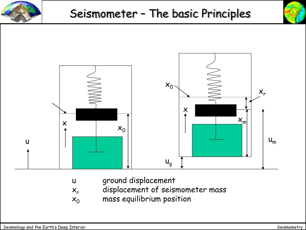
Seismometer – The basic Principles x0 xr x xm x x0 um u ug u ground displacement xr displacement of seismometer mass x0 mass equilibrium position
x0 xr x ug Seismometer – The basic Principles The motion of the seismometer mass as a function of the ground displacement is given through a differential equation resulting from the equilibrium of forces (in rest): Fspring + Ffriction + Fgravity = 0 for example Fsprin=-k x, k spring constant Ffriction=-D x, D friction coefficient Fgravity=-mu, m seismometer mass . ..
x0 xr x ug Seismometer – The basic Principles using the notation introduced the equation of motion for the mass is • From this we learn that: • for slow movements the acceleration and • velocity becomes negligible, the • seismometer records ground acceleration • for fast movements the acceleration of the • mass dominates and the seismometer • records ground displacement
xr x0 x ug Seismometer – examples
xr x0 x ug Seismometer – examples
xr x0 x ug Seismometer – examples
xr x0 x ug Seismometer – examples
xr x0 x ug Seismometer – examples
xr x0 x ug Seismometer – examples
xr x0 x ug Seismometer – Questions 1. How can we determine the damping properties from the observed behavior of the seismometer? 2. How does the seismometer amplify the ground motion? Is this amplification frequency dependent? We need to answer these question in order to determine what we really want to know: The ground motion.
xr x0 x ug Seismometer – Release Test • How can we determine the damping properties from the observed behavior of the seismometer? we release the seismometer mass from a given initial position and let is swing. The behavior depends on the relation between the frequency of the spring and the damping parameter. If the seismometers oscillates, we can determine the damping coefficient h.
xr x0 x ug Seismometer – Release Test
xr x0 x ug Seismometer – Release Test The damping coefficients can be determined from the amplitudes of consecutive extrema ak and ak+1 We need the logarithmic decrement L ak ak+1 The damping constant h can then be determined through:
T ak xr x0 ak+1 x ug Seismometer – Frequency The period T with which the seismometer mass oscillates depends on h and (for h<1) is always larger than the period of the spring T0:
xr x0 x ug Seismometer – Response Function 2. How does the seismometer amplify the ground motion? Is this amplification frequency dependent? To answer this question we excite our seismometer with a monofrequent signal and record the response of the seismometer: the amplitude response Ar of the seismometer depends on the frequency of the seismometer w0, the frequency of the excitation w and the damping constant h:
xr x0 x ug Seismometer – Response Function
Sampling rate Sampling frequency, sampling rate is the number of sampling points per unit distance or unit time. Examples?
Data volumes Real numbers are usually described with 4 bytes (single precision) or 8 bytes (double precision). One byte consists of 8 bits. That means we can describe a number with 32 (64) bits. We need one switch (bit) for the sign (+/-) -> 32 bits -> 231 = 2.147483648000000e+009 (Matlab output) -> 64 bits -> 263 = 9.223372036854776e+018 (Matlab output) (amount of different numbers we can describe) • How much data do we collect in a typical seismic experiment? • Relevant parameters: • Sampling rate 1000 Hz, 3 components • Seismogram length 5 seconds • 200 Seismometers, receivers, 50 profiles • 50 different source locations • Single precision accuracy • How much (T/G/M/k-)bytes to we end up with? What about compression?
(Relative) Dynamic range What is the precision of the sampling of our physical signal in amplitude? Dynamic range: the ratio between largest measurable amplitude Amax to the smallest measurable amplitude Amin. The unit is Decibel (dB) and is defined as the ratio of two power values (and power is proportional to amplitude square) In terms of amplitudes Dynamic range = 20 log10(Amax/Amin) dB Example: with 1024 units of amplitude (Amin=1, Amax=1024) 20 log10(1024/1) dB 60 dB
Nyquist Frequency (Wavenumber, Interval) The frequency half of the sampling ratedt is called the Nyquist frequency fN=1/(2dt). The distortion of a physical signal higher than the Nyquist frequency is called aliasing. The frequency of the physical signal is > fN is sampled with (+) leading to the erroneous blue oscillation. What happens in space? How can we avoid aliasing?
Signal and Noise Almost all signals contain noise. The signal-to-noise ratio is an important concept to consider in all geophysical experiments. Can you give examples of noise in the various methods?
Discrete Convolution Convolution is the mathematical description of the change of waveform shape after passage through a filter (system). There is a special mathematical symbol for convolution (*): Here the impulse response function g is convolved with the input signal f. g is also named the „Green‘s function“
Convolution Example(Matlab) Impulse response >> x x = 0 0 1 0 >> y y = 1 2 1 >> conv(x,y) ans = 0 0 1 2 1 0 System input System output
Convolution Example (pictorial) x „Faltung“ y y x*y 0 1 0 0 0 1 2 1 0 1 0 0 0 1 2 1 0 1 0 0 1 1 2 1 0 1 0 0 2 1 2 1 0 1 0 0 1 1 2 1 0 1 0 0 0 1 2 1
Deconvolution Deconvolution is the inverse operation to convolution. When is deconvolution useful?
Digital Filtering • Often a recorded signal contains a lot of information that we are not interested in (noise). To get rid of this noise we can apply a filter in the frequency domain. • The most important filters are: • High pass: cuts out low frequencies • Low pass: cuts out high frequencies • Band pass: cuts out both high and low frequencies and leaves a band of frequencies • Band reject: cuts out certain frequency band and leaves all other frequencies
Seismic Noise Observed seismic noise as a function of frequency (power spectrum). Note the peak at 0.2 Hz and decrease as a distant from coast.