Woodblock Print, from “Thirty-Six Views of Mt. Fuji”, by K. Hokusai, ca. 1830

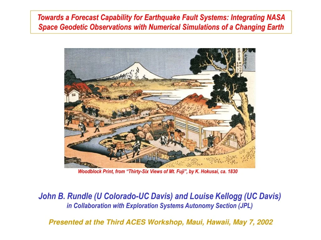
1. Towards a Forecast Capability for Earthquake Fault Systems: Integrating NASA Space Geodetic Observations with Numerical Simulations of a Changing Earth Woodblock Print, from “Thirty-Six Views of Mt. Fuji”, by K. Hokusai, ca. 1830 John B. Rundle (U Colorado-UC Davis) and Louise Kellogg (UC Davis) in Collaboration with Exploration Systems Autonomy Section (JPL) Presented at the Third ACES Workshop, Maui, Hawaii, May 7, 2002

2. Development of the Virtual_California Simulation P. B. Rundle, J.B. Rundle, K.F. Tiampo, J. Sa Martins, S. McGinnis and W. Klein, Nonlinear network dynamics on earthquake fault systems, Phys. Rev. Lett., v. 87, n. 14, p. 148501, October 1 (2001). J.B. Rundle, P. B. Rundle, W. Klein, J. Sa Martins, K.F. Tiampo, A. Donnellan and L.H. Kellogg, GEM plate boundary simulations for the plate boundary observatory: Understanding the physics of earthquakes on complex fault systems, PAGEOPH, in press (2001). P. B. Rundle, J.B. Rundle, J. Sa Martins, K.F. Tiampo, S. McGinnis, W. Klein, Triggering dynamics on earthquake fault systems, pp. 305-317, Proc. 3rd Conf. Tect. Problems San Andreas Fault System, Stanford University (2000). P. B. Rundle, J.B. Rundle, J. Sa Martins, K.F. Tiampo, S. McGinnis, W. Klein, Network dynamics of Earthquake Fault Systems, Trans. Am. Geophys. Un. EOS, 81 (48) Fall Meeting Suppl. (2000)

3. The Virtual_California Simulation: Characteristics & Properties Backslip model -- Stress is always finite and bounded. Stress accumulation on each fault due to plate tectonics is linear in time, but interactions may cause effectively produce time- dependent stress accumulation. Linear interactions (stress transfer) -- At the moment, interactions are purely elastic, but viscoelastic interactions are possible also. Arbitrarily complex fault system topologies -- At the moment, all faults are vertical strike-slip faults. Boundary element mesh is ~ 10 km horizontal, 20 km vertical. Faults are embedded in an elastic half space, but layered media are possible as well. Friction laws are based on laboratory experiments of Tullis-Karner- Marone, with additive stochastic noise. Method of solution for stochastic equations is therefore via Cellular Automaton methods. Friction laws based on general theoretical law obtained by Klein et al. (1997), special cases of which are TKM and rate-and-state friction.

4. F Baseline values for parameters  are determined for each fault segment. It can easily be shown that: 2 = So  is an observable quantity. Deng and Sykes (1997) tabulate the average fraction of stable interseismic, aseismic slip for many faults in California.  > 0 Stress R Time F  = 0 Stress,  R Data from T Tullis, PNAS, 1996 Average stable aseismic slip Total slip Remarks on Friction: Aseismic Slip (“Stress Leakage”) Factor   determines fraction of total slip that is stable aseismic slip.

5. The historic record of earthquakes over the last 200 years is shown at left. At right is the model fault system used for the simulations. At right is a representation of the fault friction encoded via data assimilation of historic events Fault Network Model for Southern California Dynamics of Earthquakes: Simulations See for example J.B.R. et al., Phys. Rev. E, 61, 2418 (2000); P.B. Rundle et al., Phys. Rev. Lett., 87, 148501 (2001). Historic Earthquakes: Last 200 Years  = CFF Stress: Time vs. Space Simulations of earthquake fault systems can be carried out using the Virtual California (GEM) model. At left is shown the buildup of CFF stress over time and space. Lines = Earthquakes Time (Years) Space (Fault Segments) At right is shown an example of one of the large earthquakes that occur during a simulation. San Andreas Fault

6. Surface Deformation from Earthquakes There is a wealth of data characterizing the surface deformation observed following earthquakes. As an example, we show data from the October 16, 1999 Hector Mine event in the Mojave Desert of California (left), along with the simulations from the Virtual California simulation (right). At left is a map of the surface rupture. Below is the surface displacement observed via GPS (left) and via Synthetic Aperature Radar Interferometry, “InSAR” (right). At right is a map of the simulated event shown earlier. Below are the associated GPS-type (left) and the InSAR-C-type (right) surface displacements. InSAR (JPL) GPS (JPL)

7. Difference: Pre minus Post Anomalous Precursory Sliding We can look at the anomalous slip that is precursory to the large earthquake at 701543, and compare it to any anomalous slip following the event. We can use GPS-type measurements as well as InSAR At right is a map of 5 years preceeding the main shock (left panel), as well as the 5 years following (right panel). With GPS vectors, it is difficult to observe precursory signals. Notice that there are smaller several pre-shocks At left are the same deformation fields as seen in the GPS vectors above, but displayed assuming C-Band InSAR. The elastic effects of the pre-shocks can easily be seen, and tend to obscure the anomalous pre-slip. In the slide at left below, we remove elastic effects of the pre-shocks.

8. A Comparison at C-Band:InSAR Difference Fringes Tend to Define the Rupture Extent The difference fringes are small (red = positive and blue= negative regions), and are concentrated along the portions of the San Andreas that are about to initiate sliding, either in the main shock or the pre-and post-shocks.

9. The difference fringes are small (red = positive and blue= negative regions), and are concentrated along the portions of the San Andreas that are about to initiate sliding, either in the main shock or the pre-and post-shocks. A Comparison at L-Band:InSAR Difference Fringes Tend to Define the Rupture Extent

10. Detecting Critical Fluctuations from Surface Data Defining a “Local Ginzburg Criterion” or “Squared Normalized Strain Rate” If large earthquakes are examples of critical phenomena, then we should expect to observe large fluctuations in all observables prior to failure. In the study of critical phenomena, these fluctuations are measured by the “Ginzburg Criterion”, the ratio of the variance in an observable field variable to the square of the mean. Building upon this idea, we define a “Local Ginzburg Criterion - (LGC)” for surface shear strain rate along faults: LGC  [ Strain Rate at (x,t) / Time - Averaged Strain Rate at x ] 2 LGC can be regarded as the squared normalized strain rate.

11. Comparing the CFF (Left) and LGC (Right) Observable Unobservable Here we show a scheme that effectively “maps” the LGC into the CFF. At time t, we compile a histogram of values of the variable:   Log10 [1 + LGC(x,t) ] at time t. The histogram resembles an exponential distribution with standard deviation . We assign the color “blue” to the value  = 0, and the color “red” to all values of  > .5 , with other spectral colors between. The result is a time-space image that appears to “map” the observable LGC into the unobservable CFF. Using simulations, it may be possible to define and evaluate a number of such mappings.

12. Fault ~ 1 Km Strain Arrays -- Important to Measure Strain Directly Not by Differencing Displacement Vectors It is important to measure strain directly, not by differencing displacement vectors, to eliminate noise effects. Advantages of strain arrays: 1. Common atmosphere 2. Common electronic noise 3. Redundancy Can be done either with GPS or precisely registered InSAR images.

13. Finite Element Models of Blind Thrusts Methodology: Finite Element Models (FEM) using JPL’s GeoFEST/VISCO 3-D Software (Allows realistic rheology and structure, including faults). Work in progress includes: Layered crust and upper mantle with a low rigidity basin representing possible fault systems in the LA Basin. All models include the San Andreas fault, the Sierra Madre thrust All models include downwelling beneath the Transverse Ranges and shortening across the basin. We compare models that include only the San Andreas and Sierra Madre faults (SAF + SMF) Near term goals: Develop models of the surface deformation resulting from different models of earth structure. Specifically, we are interested in the ability of an InSAR mission to distinguish deformation resulting from blind thrusts that may be otherwise difficult to identify: A daylighting thrust fault in addition to the SAF + SMF A blind thrust fault in addition to the SAF + SMF

14. Fault Geometry in Three Comparative 2-D Models Models include shortening and downwelling Models extend 400 km laterally And 100 deep Daylighting Thrust Model Blind Thrust Model

15. Vertical deformation in 3 FEM models using GeoFEST

16. Conclusions About Model-Based Forecasting Our results indicate that: It will be important to detect differences at the mm/y level to observe anomalous effects precursory to large earthquakes. With noisy systems, this will be difficult. So...We must think in terms of systems that observe strain directly...not as differences of deformation vectors. We will need the spatial resolution and coverage that only InSAR can provide. Our ongoing work is aimed at: Developing other measures of strain that are readily observable and that mirror the underlying stress-strain dynamics.