3D Geometry for Computer Graphics Class 7: SVD Basics and Applications
Explore the geometry of linear transformations, spectral decomposition, SVD, shape matching, animation compression, and eigenfaces in computer graphics. Learn how SVD is crucial in linear algebra and its applications in animation compression and shape matching. Discover how eigenfaces assist in face recognition through principal component analysis. Uncover the importance of dimensionality reduction in handling vast animation data. Find out about non-linear dimensionality reduction methods for complex datasets.


3D Geometry for Computer Graphics Class 7: SVD Basics and Applications
E N D
Presentation Transcript
3D Geometry forComputer Graphics Class 7
The plan today • Review of SVD basics • Connection PCA • Applications: • Eigenfaces • Animation compression
The geometry of linear transformations A • A linear transform A always takes hyper-spheres to hyper-ellipses. A
The geometry of linear transformations A • Thus, one good way to understand what A does is to find which vectors are mapped to the “main axes” of the ellipsoid. A
Spectral decomposition • If we are lucky: A = V VT, V orthogonal • The eigenvectors of A are the axes of the ellipse A
Spectral decomposition • The standard basis: y x Rotation VT Au = V VTu
Spectral decomposition • Scaling: x’’ = 1 x’, y’’ =2 y’ Scale Au = V VTu
Spectral decomposition • Rotate back: Rotate V Au = V VTu
General linear transformations: SVD • In general A will also contain rotations, not just scales: 1 1 1 2 A
SVD • The standard basis: y x Rotation VT Au = U VTu
Spectral decomposition • Scaling: x’’ = 1x’, y’’ =2y’ Scale Au = U VTu
Spectral decomposition • Rotate again: Rotate U Au = U VTu
SVD more formally • SVD exists for any matrix • Formal definition: • For square matrices A Rnn, there exist orthogonal matrices U, V Rnn and a diagonal matrix , such that all the diagonal values i of are non-negative and =
Reduced SVD • For rectangular matrices, we have two forms of SVD. The reduced SVD looks like this: • The columns of U are orthonormal • Cheaper form for computation and storage Mn Mn nn nn =
Full SVD • We can complete U to a full orthogonal matrix and pad by zeros accordingly Mn MM Mn nn =
SVD is the “working horse” of linear algebra • There are numerical algorithms to compute SVD. Once you have it, you have many things: • Matrix inverse can solve square linear systems • Numerical rank of a matrix • Can solve least-squares systems • PCA • Many more…
SVD is the “working horse” of linear algebra • Must remember: SVD is expensive! • For a nn matrix, SVD costs O(n3). • For sparse matrices could sometimes be cheaper
Shape matching • We have two objects in correspondence • Want to find the rigid transformation that aligns them
Shape matching • When the objects are aligned, the lengths of the connecting lines are small.
Shape matching – formalization • Align two point sets • Find a translation vector t and rotation matrix R so that:
Summary of rigid alignment = H is 22 or 33 matrix! • Translate the input points to the centroids: • Compute the “covariance matrix” • Compute the SVD of H: • The optimal rotation is • The translation vector is
SVD for animation compression Chicken animation
3D animations • Each frame is a 3D model (mesh) • Connectivity – mesh faces
3D animations • Each frame is a 3D model (mesh) • Connectivity – mesh faces • Geometry – 3D coordinates of the vertices
3D animations • Connectivity is usually constant (at least on large segments of the animation) • The geometry changes in each frame vast amount of data, huge filesize! 13 seconds, 3000 vertices/frame, 26 MB
Animation compression by dimensionality reduction • The geometry of each frame is a vector in R3N space (N = #vertices) 3N f
Animation compression by dimensionality reduction • Find a few vectors of R3N that will best represent our frame vectors! VTff ff U 3Nf VT =
Animation compression by dimensionality reduction VT • The first principal components are the important ones u1 u2 u3 =
Animation compression by dimensionality reduction • Approximate each frame by linear combination of the first principal components • The more components we use, the better the approximation • Usually, the number of components needed is much smaller than f. u3 u1 u2 1 + 2 + 3 =
Animation compression by dimensionality reduction ui • Compressed representation: • The chosen principal component vectors • Coefficients i for each frame Animation with only 2 principal components Animation with 20 out of 400 principal components
Eigenfaces • Same principal components analysis can be applied to images
Eigenfaces • Each image is a vector in R250300 • Want to find the principal axes – vectors that best represent the input database of images
Reconstruction with a few vectors • Represent each image by the first few (n) principal components
Face recognition • Given a new image of a face, w R250300 • Represent w using the first n PCA vectors: • Now find an image in the database whose representation in the PCA basis is the closest: The angle between w and w’ is the smallest w w’ w w’
Non-linear dimensionality reduction • More sophisticated methods can discover non-linear structures in the face datasets Isomap, Science, Dec. 2000