Debates on Macroeconomic Policy
310 likes | 509 Vues
Debates on Macroeconomic Policy. By: Jeff, Billy, Chris T, Yuki, Chris H. * Day 1 Focus *. Demand-pull inflation, and the tradeoffs between inflation and unemployment as expressed by the Phillips Curve Cost-push inflation and stagflation

Debates on Macroeconomic Policy
E N D
Presentation Transcript
Debates on Macroeconomic Policy By: Jeff, Billy, Chris T, Yuki, Chris H
* Day 1 Focus * • Demand-pull inflation, and the tradeoffs between inflation and unemployment as expressed by the Phillips Curve • Cost-push inflation and stagflation • Wage and price controls, and wage and price guidelines
Demand-Pull Inflation • Caused by increase in aggregate demand • inflation increases and unemployment decreases • Increase in aggregate demand increases inflation and output • Increase in output lower unemployment and higher wages • Increase in wages further increases inflation • Can be shown using a Phillips curve
Demand-Pull Inflation Page.444
The Phillips Curve • Keynesian economist A.W.H. Phillips believed inverse relationship between inflation and unemployment was predictable • Created the curve called the Phillips curve • Government could use curve to predict how policy would affect the economy
The Phillips Curve Page.445
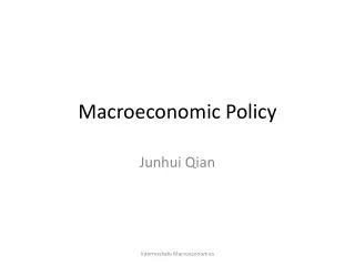
Shifts in the Phillips Curve Page.446
Cost-Push Inflation • Caused by decreases in aggregate supply, due to increase in input prices • Cost of production increases higher inflation and less output • Less output higher unemployment • Inflation and unemployment have direct relationship, as both increase at same time, called stagflation (worst-case scenario)
Cost-Push Inflation Page.447
Wage and Price Policies • Attempted by government in 1970s and 1980s to solve stagflation • Consisted of wage and price controls, and wage and price guidelines
Wage and Price Guidelines • Implemented from 1969-1975 • Government encouraged voluntary caps on wages and prices by labour unions and businesses • Businesses and labour unions were un-cooperative • Inflation was 5% when the commission was formed in 1969, and rose to 10% by 1975 • Ineffective at battling inflation
Wage and Price Controls • Implemented in 1975 • Wages and salaries were only allowed to increase by a maximum percentage each year (wages could increase by max of 8% in 1976, 6% in 1977, and 4% in 1978) • Businesses allowed price increases only to cover increase in costs, and restrictions put on profits • Inflation dropped during the next three years from 10% in 1975, to between 7.5-9% from 1976-1978, but rose above 10% by 1980, two years after wage and price controls were lifted
Debate Over Wage and Price Policies • Opposition to policies because they are ineffective, unfair, and inefficient • Ineffective because wage and price guidelines are voluntary are unsuccessful at decreasing inflation, and wage and price controls only work in short run but inflation rises again once the controls have been removed • Unfair because some sectors are easier to regulate than others and wage and price controls cannot be universally applied, so people in some sectors will have limited wage increases, and others will not. • Inefficient because wage and price controls are similar to price ceilings, so price cannot be used to gauge changes in supply and demand, and resources may be allocated to inefficient businesses rather than those who run more efficently
Day One Summary • Demand-Pull Inflation • The Phillips Curve • Cost-Push Inflation • Wage and Price Policies
Day 2 Focus • Monetarism: • -central equations (velocity of money, equation of exchange, quantity of money) • -inflationary rates and monetary growth • -monetarist policies • -the monetary rule • Supply-Side Economics: • -reduction in incentives • -focus on aggregate supply • -the Laffer curve • -the influence of supply side economics
Monetarism • An economic perspective that emphasizes the influence of money on the economy and the ability of private markets to accommodate fluctuations in economy
Monetarists versus Keynesians • Oppose fiscal policies preferred Keynesians, instead favour monetary policies • Monetarists agree that economy is susceptible to shocks, but misguided government intervention only worsens situation • Believe unwise use of monetary policy is mostly to blame for shocks in economy
The Velocity of Money (V) • Concept that is central to monetarism • Velocity of money (V) = nominal GDP money supply (M) • Velocity of money (V): the average # of times money is spent on final goods and services during a year • Nominal GDP: total dollar value of final goods and services produced in economy • Money supply (M) = M1 (publicly held currency and publicly held deposits, excluding cash reserves) EX1: If Canada’s nominal GDP is $800 billion, and M1 is $ 50 billion, what is the velocity?
The Equation of Exchange • Nominal GDP = V x M • GDP expresses both price level (P) and output (Q) • Nominal GDP = P x Q EX2: $800 billion = 2.0 x $400 billion • V x M = P x Q Using EX1 and EX2: $50 billion x 16 = 2.0 x $400 billion
The Quantity of Money • The velocity of money changes over time due to long-run factors, almost constant in short run • Real output varies slightly from potential level in short run, wages are flexible so economy adjusts to changes in prices or unemployment (after a brief period of inflexible wages) • Velocity of money and real output are reasonably stable, so V* and Q* are set as constant values • M x V* = P x Q* • Result is direct relationship between money and prices
Inflation Rates and Monetary Growth • Extension of quantity theory of money that shows relationship between inflation rates and growth in money supply • When both velocity and real output are constant, the percentage changes in money supply and in price level are equal • % in M = % in P • Velocity of money and real output are not perfectly constant, so inflation is not always identical to the rate of monetary growth, but they will be close
Inflation Rates and Monetary Growth – EXAMPLE M x V* = P x Q* $50 billion x 16 = 2.0 x $400 billion $55 billion x 16 = 2.2 x $400 billion • % in M = ($55 billion - $50 billion) x 100 % $50 billion = 10 % • % in P = (2.2 – 2.0) x 100% 2.0 = 10%
Monetarist Policies • Money is the key factor in the economy, unlike Keynesians who believe it is only one of many factors • Fiscal policy has little influence due to “crowding out effect” • Even monetary policy cannot change output from its potential level • Only way to stabilize economy is minimizing harmful effects of inflation, when bank of Canada minimizes rate of growth of money supply
The Monetary Rule • The monetary rule forces central banks to increase the money supply by a constant rate each year • Recommended at 3% based on real long-term growth in economy
Supply-Side Economics • Focuses on influence of production costs on prices and incomes • Influence on aggregate supply is most important result of government policy
Reduction in Incentives • Recent government has impaired economic activity by reducing incentives to be productive • Personal Income and Business Taxes: When taxes increase, disposable income falls • Sales Taxes: Reduces amount of products that can be bough with a given disposable income • Transfers and Subsidies: welfare, Unemployment Insurance, and farm subsidies diminish incentives to generate private income • Regulation: Environmental, safety…regulations have all increased business costs and reduced incentives to invest
Focus on Aggregate Supply • More taxes and government regulation decrease aggregate supply, and the AS curve shifts to the left • Same as cost-push inflation; increased costs push up prices a the same time that unemployment rises stagflation • Supply-siders call for tax cuts and deregulation to lower prices and unemployment
The Laffer Curve • Demonstrates an assumed relationship between tax rates and tax revenues • Tax rates and tax revenues have direct relationship at low tax rates, therefore tax increase at lower tax rates also increases tax revenues, and positive slope on graph • Tax rates and tax revenues have indirect relationship at high tax rates, therefore a tax increase at higher tax rates decreases tax revenues, and negative slope on graph • Tax increases at higher tax rates have dampening effect on economic activity