LECTURE 12: REESTIMATION, EM AND MIXTURES

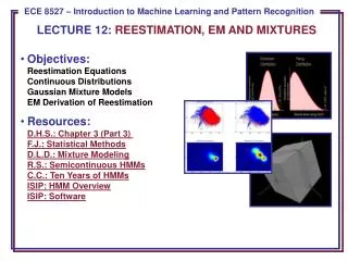
1. LECTURE 12: REESTIMATION, EM AND MIXTURES • Objectives:Reestimation EquationsContinuous DistributionsGaussian Mixture ModelsEM Derivation of Reestimation • Resources:D.H.S.: Chapter 3 (Part 3) F.J.: Statistical MethodsD.L.D.: Mixture ModelingR.S.: SemicontinuousHMMsC.C.: Ten Years of HMMsISIP: HMM OverviewISIP: Software

2. Evaluation and Decoding (Review)

3. Problem No. 3: Learning • Let us derive the learning algorithm heuristically, and then formally derive it using the EM Theorem. • Define a backward probability analogous to αi(t): • This represents the probability that we are in state ωi(t) and will generate the remainder of the target sequence from [t+1,T]. • Define the probability of a transition from ωi(t-1) to ωi(t) given the model generated the entire training sequence, vT: • The expected number of transitions from ωi(t-1) to ωi(t) at any time is simply the sum of this over T: .

4. Problem No. 3: Learning (Cont.) • The expected number of any transition from ωi(t) is: • Therefore, a new estimate for the transition probability is: • We can similarly estimate the output probability density function: • The resulting reestimation algorithm is known as the Baum-Welch, or Forward Backward algorithm: • Convergence is very quick, typically within three iterations for complex systems. • Seeding the parameterswith good initial guessesis very important. • The forward backward principle is used in many algorithms.

5. Continuous Probability Density Functions • The discrete HMM incorporates adiscrete probability densityfunction, captured in the matrix B, to describe the probability of outputting a symbol. • Signal measurements, or featurevectors, are continuous-valued N-dimensional vectors. • In order to use our discrete HMM technology, we must vector quantize (VQ) this data – reduce the continuous-valued vectors to discrete values chosen from a set of M codebook vectors. • Initially most HMMs were based on VQ front-ends. However, for the past 30 years, the continuous density model has become widely accepted. • We can use a Gaussian mixture model to represent arbitrary distributions: • Note that this amounts to assigning a mean and covariance matrix for each mixture component. If we use a 39-dimensional feature vector, and 128 mixtures components per state, and thousands of states, we will experience a significant increase in complexity  … 0 1 2 3 6 4 5

6. Continuous Probability Density Functions (Cont.) • It is common to assume that the features are decorrelated and that the covariance matrix can be approximated as a diagonal matrix to reduce complexity. We refer to this as variance-weighting. • Also, note that for a single mixture, the log of the output probability at each state becomes a Mahalanobis distance, which creates a nice connection between HMMs and PCA. In fact, HMMs can be viewed in some ways as a generalization of PCA. • Write the joint probability of the data and the states given the model as: • This can be considered the sum of the product of all densities with all possible state sequences, ω, and all possible mixture components, K: • and

7. Application of EM • We can write the auxiliary function, Q, as: • The log term has the expected decomposition: • The auxiliary function has three components: • The first term resembles the term we had for discrete distributions. The remaining two terms are new:

8. Reestimation Equations • Maximization of requires differentiation with respect to the parameters of the Gaussian: . This results in the following: • where the intermediate variable, , is computed as: • The mixture coefficients can be reestimated using a similar equation:

9. Case Study: Speech Recognition InputSpeech • Based on a noisy communication channel model in which the intended message is corrupted by a sequence of noisy models • Bayesian approach is most common: • Objective: minimize word error rate by maximizing P(W|A) • P(A|W): Acoustic Model • P(W): Language Model • P(A): Evidence (ignored) • Acoustic models use hidden Markov models with Gaussian mixtures. • P(W) is estimated using probabilisticN-gram models. • Parameters can be trained using generative (ML)or discriminative (e.g., MMIE, MCE, or MPE) approaches. AcousticFront-end Acoustic ModelsP(A/W) Language ModelP(W) Search Recognized Utterance

10. Case Study: Acoustic Modeling in Speech Recognition

11. Case Study: Fingerspelling Recognition

12. Case Study: Fingerspelling Recognition

13. Summary • Hidden Markov Model: a directed graph in which nodes, or states, represent output (emission) distributions and arcs represent transitions between these nodes. Emission distributions can be discrete or continuous. • Continuous Density Hidden Markov Models (CDHMM): the most popular form of HMMs for many signal processing problems. Gaussian mixture distributions are commonly used (weighted sum of Gaussian pdfs). • Subproblems: Practical implementations of HMMs require computationally efficient solutions to: • Evaluation: computing the probability that we arrive in a state a time t and produce a particular observation at that state. • Decoding: finding the path through the network with the highest likelihood (e.g., best path). • Learning: estimating the parameters of the model from data. • The EM algorithm plays an important role in learning because it proves the model will converge if trained iteratively. • There are many generalizations of HMMs including Bayesian networks, deep belief networks and finite state automata. • HMMs are very effective at modeling data that has a sequential structure.