Advancements in Scalable Solvers for Petascale Electromagnetic Simulations
This document presents an overview of scalable solvers used in petascale electromagnetic simulations, particularly at the SLAC and Lawrence Berkeley National Laboratory. It examines shape determination and optimization for superconducting RF cavities, highlighting metrics like mode frequencies and field distributions. Furthermore, it covers ongoing developments in linear and nonlinear eigensolvers designed to handle complex eigenvalue problems while improving scalability and performance. Future work aims to refine algorithms, incorporate more parameters, and enhance simulation capabilities in cryomodule RF units.

Advancements in Scalable Solvers for Petascale Electromagnetic Simulations
E N D
Presentation Transcript
Lie-Quan (Rich) Lee, Volkan Akcelik, Ernesto Prudencio, Lixin Ge Stanford Linear Accelerator Center Xiaoye Li, Esmond Ng Lawrence Berkeley National Laboratory Scalable Solvers in Petascale Electromagnetic Simulation Work supported by DOE ASCR, BES & HEP Divisions under contract DE-AC02-76SF00515 COMPASS All-hands Meeting, Fermilab, Sept. 17-18 2007
Overview • Shape Determination/Optimization • V. Akcelik, L. Lee (SLAC) • T. Tautges, P. Knupp, L. Diachin (ITAPS) • O. Ghattas, E. Ng, D. Keyes (TOPS) • Linear and Nonlinear Eigensolvers • L. Lee(SLAC), X. Li, E. Ng, C. Yang (LBNL/TOPS) • Scalable Linear Solvers • L. Lee (SLAC), X. Li, E. Ng (TOPS)
Shape Determination and Optimization For SCRF Cavities • Shape changes due to • Fabrication errors • Addition of stiffening rings • Tuning for accelerating mode • Change HOM Damping -> Beam quality HOM Damping changes Ring in the middle Tuning
Least-squares Minimization • Unknowns are shape deviation parameters • Gauss-Newton with truncated-SVD • Indefinite linear systems from KKT (deferred) Its forward problem is Maxwell eigenvalue problem
Example 1 for ILC TDR Cavity • Create a synthetic example, artificially deform a 3D 9 cell ILC cavity. • Choose a set of parameters defining shape variations, in total 26 independent inversion parameters. • Cell radius dr (x9) an cell length dz (x9) • Iris radius (x8) • Assign random values to these variables, and deform the cavity. • Solve the Maxwell eigenvalue problem. • Use the first 45 nonzero frequencies, and first 9 modes field distribution as the targeted values
Results for Example 1 • The nonlinear solver converges within a handful of iterations • Frequencies and Fields match remarkably • Objective function decreases by 10e6 • The “target” and “inverted” cavity shapes are very close to each other
Determining TDR Shape with Measured Frequencies • Experimental data for manufactured baseline ILC cavities from DESY • The first 45 mode frequencies, and the first 9 monopole mode field distribution along the cavity axis • 82 parameters: cell radius, length, tuning, warping, and iris radius Cell radius error Deformed surface Elliptical shape Cell length error
Results • Difference of Frequencies and Field values • Red: inverted cavity - measured values • Black/blue: ideal shape - measured values MHz • An article has been accepted by JCP
Future Work on Shape Determination • Measurement data contain error • better algorithm • Choices of shape deviation parameters • Extending the method to using frequencies, fields and external Qs where • The forward problem is a complex nonlinear eigenvalue problem! • Mesh smoothing (ITAPS) Meshes near pickup gap red: deformed black: original
RF Cavity Eigenvalue Problem E Closed Cavity M Nedelec-type Element Find frequency and field vector of normal modes: “Maxwell’s Eqns in Frequency Domain”
Cavity with Waveguide Coupling • One waveguide mode per port only Waveguide BC Waveguide BC Open Cavity Waveguide BC • Vector wave equation with waveguide boundary conditions can be modeled by a non-linear eigenvalue problem With
Cavity with Waveguide Coupling for Multiple Waveguide Modes Waveguide BC Waveguide BC Open Cavity Waveguide BC • Vector wave equation with waveguide boundary conditions can be modeled by a non-linear eigenvalue problem (NEP) where
Physics Problems and Solver Options Krylov Subspace Methods Domain-specific preconditioners Omega3P Lossless Lossy Material Periodic Structure External Coupling ISIL w/ refinement ESIL/with Restart Implicit/Explicit Restarted Arnoldi SOAR Self-Consistent Iteration Nonlinear Arnoldi/JD i WSMP MUMPS SuperLU_Dist Different solver options have different performance dynamics
Path to Simulate ILC RF Unit (3-cryomodule) • Optimized ILC single cavity routinely • Simulated 4-cavity STF last year • Simulating 8-cavity ILC Cryomodule this year • Simulate ILC 3-cryomodule RF Unit - ~200M DOFs, further CS/AM advance needed, petascale
Future Work for Eigensolvers • Parallelize AMLS, understand and improve its performance and scalability • Nonlinear Jacobi-Davidson • Choice of initial space • Strategy for updating preconditioner and choice of preconditioners • New algorithm development for NEP/LEP • avoid shift-invert for interior eigenvalues • LEP helps NEP (Self Consistent Iterations)
Linear Solver is Computational Kernel of Many Codes • Indefinite Matrices • Linear systems arising from shift-invert eigensolver in Omega3P • Indefinite linear system from KKT conditions • S-parameter computation in S3P • Symmetric Positive Definite (SPD) Matrices • From implicit time-stepping in T3P • From thermal and mechanical analysis TEM3P • From electro/magneto static analysis Gun3P • Issues in Petascale Electromagnetic simulations: • Direct solver: memory usage, scalability of triangular solver • Iterative solver: performance, effectiveness (preconditioner)
Omega3P Scalability on Jaguar/XT with Iterative Linear Solver LCLS RF Gun • 1.5M tetrahedral elements NDOFs = 9.6M NNZ = 506M
Scalability Using Sparse Direct Solver MUMPS N=2,019,968, nnz=32,024,600 No. of entries in L =1 billion N=2M, PSPASES Triangular Solver • Sparse Direct Solver is effective for highly indefinite matrices • Scalability affected by performance of Triangular Solver • Need more scalable Triangular Solvers
More “Memory-usage” Scalable Sparse Direct Solvers MUMPS per-rank memory usage N=1.11M, nnz=46.1M Complex matrix • Maximal per-rank MU is 4-5 times than the average MU • Once it cannot fit into Nprocs, it most likely will not fit into 2*Nprocs • More “memory-usage” scalable solvers needed
Memory Saving Techniques • Single precision for factor matrix, iterative refinement to recover double precision accuracy (F) • Domain-specific Preconditioners • Factorize real part of the matrix (R) • Real part is a good approximation to the complex matrix • User single precision to factorize real part of the matrix (RF) • Hierarchical preconditioners (FE order is the level) (HP) • single precision for (1,1)-block (HPF) • real part only for (1,1)-block (HPR) • single precision & real part for (1,1)-block (HPRF)
Recent Progress of SuperLU(Xiaoye Li) Parallel symbolic factorization significantly reduces memory usage Matrix for DDS Matrix for ILC Cavity
Future Work on Linear Solvers • Direct versus iterative solvers, hybrid solvers • Investigate applicability of out-of-core sparse direct solvers from TOPS • Apply multigrid solvers from TOPS for SPD matrices • Extend PSPASES to indefinite/complex matrices • Develop more effective domain-specific preconditioners