Genotype x Environment Interactions: An Essential Analysis in Agricultural Research
370 likes | 471 Vues
Learn why researchers conduct multiple experiments, what influences genotype x environment interactions, types of environments, examples of multiple experiments, determining number and location of environments, and key points for conducting analyses efficiently.

Genotype x Environment Interactions: An Essential Analysis in Agricultural Research
E N D
Presentation Transcript
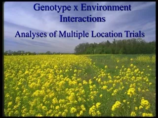
Genotype x Environment Interactions Analyses of Multiple Location Trials
Why do researchers conduct multiple experiments? • Effects of factors under study vary from location to location or from year to year. To obtain an unbias estimate. • Interest in determining the effect of factors over time. • To investigate genotype (or treatment) x environment interactions.
What are Genotype x Environment Interactions? • Differential response of genotypes to varying environmental conditions. • Delight for statisticians who love to investigate them. • The biggest nightmare for plant breeders (and some other agricultural researchers) who tryto avoid them like the plague.
A No interaction Yield B Locations
A No interaction Yield B Locations A Cross-over interaction Yield B Locations
A No interaction Yield B Locations A Cross-over interaction Yield B Locations A Scalar interaction Yield B Locations
Examples of Multiple Experiments • Plant breeder grows advanced breeding selections at multiple locations to determine those with general or specific adaptability ability. • A pathologist is interested in tracking the development of disease in a crop and records disease at different time intervals. • Forage agronomist is interested in forage harvest at different stages of development over time.
Types of Environment • Researcher controlled environments, where the researcher manipulates the environment. For example, variable nitrogen. • Semi-controlled environments, where there is an opportunity to predict conditions from year to year. For example, soil type. • Uncontrolled environments, where there is little chance of predicting environment. For example, rainfall, temperature, high winds.
Why? • To investigate relationships between genotypes and different environmental (and other) changes. • To identify genotypes which perform well over a wide range of environments. General adaptability. • To identify genotypes which perform well in particular environments. Specific adaptability.
How many environments do I need? Where should they be?
Number of Environments • Availability of planting material. • Diversity of environmental conditions. • Magnitude of error variances and genetic variances in any one year or location. • Availability of suitable cooperators • Cost of each trial ($’s and time).
Location of Environments • Variability of environment throughout the target region. • Proximity to research base. • Availability of good cooperators. • $$$’s.
Points to Consider before Analyses • Normality. • Homoscalestisity (homogeneity) of error variance. • Additive. • Randomness.
Points to Consider before Analyses • Normality. • Homoscalestisity (homogeneity) of error variance. • Additive. • Randomness.
Bartlett Test(same degrees of freedom) 2n-1 = M/C M = df{nLn(S) - Ln2} Where, S = 2/n C = 1 + (n+1)/3ndf n = number of variances, df is the df of each variance
Bartlett Test(same degrees of freedom) S = 101.0; Ln(S) = 4.614
Bartlett Test(same degrees of freedom) S = 100.0; Ln(S) = 4.614 M = (5)[(4)(4.614)-18.081] = 1.880, 3df C = 1 + (5)/[(3)(4)(5)] = 1.083
Bartlett Test(same degrees of freedom) S = 100.0; Ln(S) = 4.614 M = (5)[(4)(4.614)-18.081] = 1.880, 3df C = 1 + (5)/[(3)(4)(5)] = 1.083 23df = 1.880/1.083 = 1.74 ns
Bartlett Test(different degrees of freedom) 2n-1 = M/C M = ( df)nLn(S) - dfLn2 Where, S = [df.2]/(df) C = 1+{(1)/[3(n-1)]}.[(1/df)-1/ (df)] n = number of variances
Bartlett Test(different degrees of freedom) S = [df.2]/(df) = 13.79/37 = 0.3727 (df)Ln(S) = (37)(-0.9870) = -36.519
Bartlett Test(different degrees of freedom) M = (df)Ln(S) - dfLn 2 = -36.519 -(54.472) = 17.96 C = 1+[1/(3)(4)](0.7080 - 0.0270) = 1.057
Bartlett Test(different degrees of freedom) S = [df.2]/(df) = 13.79/37 = 0.3727 (df)Ln(S) = (37)(=0.9870) = -36.519 M = (df)Ln(S) - dfLn 2 = -36.519 -(54.472) = 17.96 C = 1+[1/(3)(4)](0.7080 - 0.0270) = 1.057 23df = 17.96/1.057 = 16.99 **, 3df
Significant Bartlett Test • “What can I do where there is significant heterogeneity of error variances?” • Transform the raw data: Often ~ cw Binomial Distribution where = np and = npq Transform to square roots
Significant Bartlett Test • “What else can I do where there is significant heterogeneity of error variances?” • Transform the raw data: Homogeneity of error variance can always be achieved by transforming each site’s data to the Standardized Normal Distribution [xi-]/
Significant Bartlett Test • “What can I do where there is significant heterogeneity of error variances?” • Transform the raw data • Use non-parametric statistics
Model ~ Multiple sites Yijk = + gi + ej + geij + Eijk igi = jej = ijgeij Environments and Replicate blocks are usually considered to be Random effects. Genotypes are usually considered to be Fixed effects.
Models ~ Years and sites Yijkl = +gi+sj+yk+gsij+gyik+syjk+gsyijk+Eijkl igi=jsj=kyk= 0 ijgsij=ikgyik=jksyij = 0 ijkgsyijk = 0