Download
1 / 38
380 likes | 466 Vues
Dive into the Bs mixing observation presented by Alessandro Cerri from CERN at LBNL in 2006. Explore the last year's developments, the importance of Tevatron in flavor physics, detector advancements, benchmarks, and implications for beyond Standard Model physics.

E N D
Observation of Bs Mixing with CDF II Alessandro Cerri CERN (LBNL) Dec 11th 2006
Synopsis • Introduction • Bs mixing in the last 12 months • Flavor physics • How the Tevatron contributes • Detector • Benchmarks • Bs Mixing Observation • Is BSM physics dead? • Conclusions
What happened in the last year… • Mar 2006: D0 came out with a result based on 1fb-1 (Moriond) • Jun 2006: CDF releases a preliminary result (but not the last word) on 1fb-1 • Signal search start showing evidence • Not enough statistical power for ‘observation’ (5) • If signal is theremeasure • Sep 2006: CDF went back and improved the analysis • Signal shows up at >5 • We therefore claim observation and measurement of This last analysis will be today’s subject!
The Flavor Sector: CKM Matrix W d’ u Quarks couple to W through VCKM: rotation in flavor space! VCKM is Unitary
Last year… TeVatron contribution is critical!
The Tevatron as a b factory • (4s) B factories program extensive and very successful BUT limited to Bu,Bd • Tevatron experiments can produce all b species: Bu,Bd,Bs,Bc, B**, b,b See PRD 71, 032001 2005 • Compare to: • (4S) 1 nb (only B0, B+) • Z0 7 nb • Unfortunately • pp 100 mb b production in pp collisions is so large (~300 Hz @ 1032 cm-2 Hz) that we could not even cope with writing it to tape!
CDF and the TeVatron TOF COT Si Detector: L00,SVX II, ISL • Renewed detector & Accelerator chain: • Higher Luminosity higher event rate • Detector changes/improvements: • DAQ redesign • Improved performance: • Detector Coverage • Tracking Quality • New Trigger strategies for heavy flavors: displaced vertex trigger Delivered: 1.6 fb-1 On tape : 1.4 fb-1 Good w/o Si: 1.2 fb-1 Good w Si: 1.0 fb-1
SVT: a specialized B physics trigger The CDF Trigger ~2.7 MHz Crossing rate 396 ns clock Detector Raw Data • Level 1 • 2.7 MHz Synch. Pipeline • 5544 ns Latency • ~20 KHz accept rate Level 1 storage pipeline: 42 clock cycles Level 1 Trigger SVT L1 Accept Level 2 Trigger Level 2 buffer: 4 events • Level 2 • Asynch. 2 Stage Pipeline • ~20 s Latency • 250 Hz accept rate L2 Accept DAQ buffers L3 Farm Mass Storage (30-50 Hz) requirements • Good IP resolution • As fast as possible Customized Hardware
…and a successful endeavor! ~ 48 m Single Hit Road Detector Layers Superstrip • The recipe: specialized hardware • Clustering • Find clusters (hits) from detector ‘strips’ at full detector resolution • Template matching • Identify roads: pre-defined track templates • with coarser detector bins (superstrips) • Linearized track fitting • Fit tracks, with combinatorial limited to clusters within roads • SVT is capable of digesting >20000 evts/second, identifying tracks in the silicon • CDFII has been running it since day -1 SVT is the reason of the success and variety of B physics in CDF run II
Measure: Branching Ratios First-time measurement of many Bs and b Branching Fractions Hep-ex/0508014 Hep-ex/0502044 http://www-cdf.fnal.gov/physics/new/bottom/050310.blessed-dsd/ http://www-cdf.fnal.gov/physics/new/bottom/050310.blessed-dsd/ Hep-ex/0601003 http://www-cdf.fnal.gov/physics/new/bottom/050407.blessed-lbbr/lbrBR_cdfpublic.ps
Lifetimes: fully reconstructed hadronic modes • Testbed for our ability to understand trigger biases • Large, clean samples with understood backgrounds • Excellent mass and vertex resolution • Prerequisite for mixing fits! Efficiency (AU) (B+) = 1.661±0.027±0.013 ps (B0) = 1.511±0.023±0.013 ps (Bs) = 1.598±0.097±0.017 ps 2 3 0 1 4 Proper decay length (mm) Systematics (m) KK http://www-cdf.fnal.gov/physics/new/bottom/050303.blessed-bhadlife/
Hadronic Lifetime Results • World Average: B+ 1.653 0.014 ps-1 B0 1.534 0.013 ps-1 Bs 1.469 0.059 ps-1 Excellent agreement! ~3000 candidates
lDs Lifetime Results lifetimes measured on first 355 pb-1 compare to World Average: Bs: (1.469±0.059) ps K K Ds l l Bs
Why so much fuss around ms? • Vtdis derived from mixing effects • QCD uncertainty is factored out in this case resorting to the relative Bs/Bd mixing rate (Vtd/Vts) • Beyond the SM physics could enter in loops!
B production at the TeVatron • Production: ggbb • NO QM coherence, unlike B factories • Opposite flavor at productionone of the b quarks can be used to tell the flavor of the other at production • Fragmentation products have some memory of b flavor as well
Bs Mixing 101 Nunmix-Nmix A= Nunmix+Nmix cos(m t) A ms [ps-1] • ms>>md • Different oscillation regime Amplitude Scan Perform a ‘fourier transform’ rather than fit for frequency B lifetime Bs vs Bd oscillation
Amplitude Scan: introduction • Mixing amplitude fitted for each (fixed) value of m • On average every m value (except the true m) will be 0 • “sensitivity” defined for the average experiment [mean 0] • The actual experiment will have statistical fluctuations • Actual limit for the actual experiment defined by the systematic band centered at the measured asymmetry • Combining experiments as easy as averaging points! Just an example: Not based on real data! Is this an effective tool to search for a signal?
Bs Mixing Ingredients Proper time resolution Flavor tagging Signal-to-noise Event yield
Flavor Tagging Nright-Nwrong D= Nright+Nwrong Reconstructed decay Fragmentation product “Same Side” AmplitudeDAmplitude B meson • Flavor Taggers: • Opposite Side • Lepton (e,) • Average charge • Kaon (bcs) • Same Side: • Kaon (hadronization) Several methods, none is perfect !!!
Bs Mixing: tagging performance Measured from Bd/Bs data ~5% of the Events are effectively used!
Bs Mixing Ingredients: ct Proper time resolution
Proper time resolution BsllDs K K K K BsDs Ds l l Ds Bs Bs ~0.5% ~15% s æ ö m ç ÷ P s = s Ä s B ct Å t ç ÷ ct L K P P xy è ø t t Semileptonic modes: momentum uncertainty Fully reconstructed: Lxy uncertainty
Mixing in the real world Proper time resolution Flavor tagging power
Bs Mixing: CDF semileptonic Hep-ex/0609040 ms>16.5 @ 95% CL Sensitivity: 19.3 ps-1 Reach at large ms limited by incomplete reconstruction (ct)!
Bs Mixing: CDF hadronic Hep-ex/0609040 Total: ~8700 events! ms>17.1 @ 95% CL Sensitivity: 30.7 ps-1 This looks a lot like a signal!
Bs Mixing: combined CDF result Hep-ex/0609040 ms> 17.2 ps-1 @ 95% CL Sensitivity: 31.3 ps-1 Develop a sound statistical approach -prior to opening the box-to assess statistical significance! Minimum: -17.26 What is the probability for background to mimic this?
Likelihood Ratio Hep-ex/0609040
Likelihood Ratio Hep-ex/0609040 • Combined hadronic+semileptonic likelihoods gives 5 significance • Parabolic fit to minimum yields: • the measurement is very precise! (~2.5%) ms = 17.77 ± 0.10(stat) ± 0.07 (syst) ps-1 combined likelihoods from hadronic and semileptonic channels
Systematic Uncertainties I Hadronic Semileptonic • Mostly related to absolute value of amplitude, relevant only when setting limits • cancel in A/A, folded in confidence calculation for observation • systematic uncertainties are very small compared to statistical
Systematic Uncertainties II: ms • systematic uncertainties from fit model evaluated on toy Monte Carlo • have negligible impact • relevant systematic unc. from lifetime scale All relevant systematic uncertainties are common between hadronic and semileptonic samples
ms and Vtd • inputs: • m(B0)/m(Bs) = 0.9830 (PDG 2006) • = 1.21 +0.047 (M. Okamoto, hep-lat/0510113) • md = 0.507 ± 0.005 (PDG 2006) -0.035 |Vtd| / |Vts| = 0.2060 0.0007(exp) +0.0081 (theo) -0.0060 • compare to Belle bs (hep-ex/050679): |Vtd| / |Vts| = 0.199 +0.026 (stat) +0.018 (syst) -0.025 -0.015
ms from Tevatron & BSM Limits Hep-ph/0509117 Agashe/Papucci/Perez/Pirjol Probability
Conclusions PLB 186 (1987) 247, PLB 192 (1987) 245 PRL 62 (1989) 2233 Exciting times: • 1987 B0 mixing (UA1, Argus) • 1989 CLEO confirms B0 mixing • 1990s LEP B0 Mixing • 1993 • First time dependent md meas. (Aleph) • First lower limit on ms • 1999 CDF Run I lower limit (ms>5.8 ps-1) • 2005 • D0: ms>5.0 ps-1 • CDF: ms>7.9 ps-1 • 2006 • D0: ms [17,21] ps-1 @ 90% CL • CDF: ms=17.31+0.330.07 ps-1 • CDF: 5 observation, ms=17.77+0.100.07 ps-1 PLB 313 (1993) 498 PLB 322 (1994) 441 PRL 82 (1999) 3576 PRL 97 (2006) 021802 PRL 97 (2006) 0062003 -0.18