Download
1 / 62
620 likes | 763 Vues
CP Violation and Rare Decays in K Mesons. CP Violation in Kaon Systems in the Standard Model CP Violation in Kaon Systems Beyond the SM Why rare decays Which rare decays Conclusions.

E N D
CP Violation and Rare Decays inK Mesons • CP Violation in Kaon Systems in the Standard Model • CP Violation in Kaon Systems Beyond the SM • Why rare decays • Which rare decays • Conclusions Dipartimento di Fisica di Roma IGuido Martinelli Paris June 5th 2003
Consequences of a Symmetry p1 p3 p4 p2 [S, H] = 0 | E , p , s › We may find states which are simultaneously eigenstates of S and of the Energy CP | K10› = + | K10› CP | K20› = _| K20› sin sout ‹| K10› ‹| K20› = | KS,L0› = | K10› + | K20› if CP is conserved either =0 or =0
CP Violation in the Neutral Kaon System +- =‹+-| HW| KL › 00 =‹00| HW| KL › ‹+-| HW| KS › ‹00| HW| KS › Expanding in several “small” quantities ~ - 2 ´ ~ + ´ Conventionally: | KS › = | K1 ›CP=+1 + | K2 ›CP= - 1 | KL › = | K2 ›CP= - 1 + | K1 ›CP= + 1
Indirect CP violation: mixing HW K0 K0 HW | KL › = | K2 ›CP= - 1 CP= + 1 W s d u,c,t S=2 ( ) s d W O Box diagrams: They are also responsible for B0 - B0 mixing md,s Complex S=2 effective coupling
| | ~ CA26 sin {F(xc , xt)+ F(xt)[A24 (1- cos )] - F(xc)} BK Inami-Lin Functions + QCD Corrections (NLO) = sin = cos G2F M2W MK f2K C = 6 √2 2 MK ‹K0 | ( s (1 - 5 )d )2 | K0›= 8/3 f2K M2KBK
K0-K0 mixing in the Standard Model (and beyond) K0 | (sLA dLA) (sLB dLB) | K0 = 8/3 f2K M2K BK ()
NEW RESULTS FOR BK BNDRK(2 GeV) BK World Average by L.Lellouch at Lattice 2000 and GM 2001 0.63 0.04 0.10 0.86 0.06 0.14 CP-PACS perturbative renorm. 0.575 0.006 0.787 0.008 (quenched) DWF 0.5746(61)(191) RBC non-perturbative renorm. 0.538 0.008 0.737 0.011 (quenched) DWF SPQcdR 0.66 0.070.90 0.10 Wilson Improved NP renorm. NNC-HYP Overlap Fermions 0.66 0.040.90 0.06 perturbative Garron & al. Overlap Fermions 0.61 0.070.83 0.10 Non-perturbative Lattice 2002 preliminary
B0 - B0 mixing O B=2 Transitions ( ) H11 H12 H = H22 H21 W b d B0 B0 t HeffB=2 = b d W Hadronic matrix element (d (1 - 5 )b)2 CKM G2F M2W m2t < O > A26 Ftt () md,s = 16 2 M2W
sin 2 is measured directly from B J/ Ks decays at Babar & Belle (Bd0 J/ Ks , t) - (Bd0 J/ Ks , t) AJ/ Ks = (Bd0 J/ Ks , t) + (Bd0 J/ Ks , t) AJ/ Ks = sin 2 sin (md t)
from the study: CKM Triangle Analysis A critical review with updated experimental inputs and theoretical parameters M. Ciuchini et al . 2000 (& 2001) upgraded for ICHEP 2002-presented by A. Stocchi see also the CERN Yellow Book (CKM Workshop) similar results from Hoecker et al. 2000-2001 Dipartimento di Fisica di Roma IGuido Martinelli Paris June 5th 2003
Results for and & related quantities Allowed regions in the -plane (contours at 68% and 95% C.L.) With the constraint fromms = 0.178 0.046 = 0.341 0.028 [ 0.085 - 0.265] [ 0.288 - 0.397] at 95% C.L. sin 2 = - 0.19 0.25sin 2 = 0.695 0.056 [ -0.62 - +0.33] [ 0.68 - 0.79]
Direct CP violation: decay HW CP= + 1 | KL › = | K2 ›CP= - 1 u s K s Complex S=1 effective coupling
A0e i0= ‹ (π π)I=0IHWI K0› A2e i2= ‹ (π π)I=2IHWI K0› Where 0,2is the strong interaction phase (Watson theorem) and the weak phase is hidden in A0,2 CP if Im[A0*A2 ] 0 = i e i( 2- 0 ) [ Im A2 - ImA0] Re A2 Re A0 √2 = Re A2 / Re A0 ~1/22
In the Standard Model r = GF /(2 || Re A0 ) t = Vtd Vts* Extracting the phases: / = Im t e i(/2+2- 0 - ) r [|A0|- |A2|] 1
GENERAL FRAMEWORK HS=1 = GF/√2 Vud Vus*[(1-) i=1,2 zi (Qi -Qci) + i=1,10 (zi + yi ) Qi ] Where yi and zi are short distance coefficients, which are known in perturbation theory at the NLO (Buras et al. + Ciuchini et al.) = -Vts*Vtd/Vus*Vud We have to computeAI=0,2i= ‹ (π π)I=0,2 IQ i I K› with a non perturbative technique(lattice, QCD sum rules, 1/N expansion etc.)
New local four-fermion operators are generated Q1 = (sLA uLB) (uLB dLA) Current-Current Q2 = (sLA uLA) (uLB dLB) Q3,5 = (sRA dLA)∑q (qL,RB qL,RB) Gluon Q4,6 = (sRA dLB)∑q (qL,RB qL,RA) Penguins Q7,9 = 3/2(sRA dLA)∑q eq (qR,LB qR,LB) Electroweak Q8,10 = 3/2(sRA dLB)∑q eq (qR,LB qR,LA) Penguins + Chromomagnetic end electromagnetic operators to be discussed in the following
A0 = ∑i Ci() ‹ (π π)IQi () I K ›I=0 (1- IB) = renormalization scale -dependence cancels if operator matrix elements are consistently computed ISOSPIN BREAKING A2 = ∑i Ci() ‹ (π π)IQi () I K ›I=2 IB = 0.25 0.08 (Munich from Buras & Gerard) 0.25 0.15 (Rome Group) 0.16 0.03 (Ecker et al.) 0.10 0.20 Gardner & Valencia, Maltman & Wolf, Cirigliano & al.
100 GeV Large mass scale: heavy degrees of freedom (mt , MW, Ms ) are removed and their effect included in the Wilson coefficients perturbative region renormalizazion scale (inverse lattice spacing 1/a); this is the scale where the quark theory is matched to the effective hadronic theory 1-2 GeV non-perturbative region Scale of the low energy process ~ MW THE SCALE PROBLEM: Effective theories prefer low scales, Perturbation Theory prefers large scales
if the scale is too low problems from higher dimensional operators (Cirigliano, Donoghue, Golowich) - it is illusory to think that the problem is solved by using dimensional regularization on the lattice this problem is called DISCRETIZATION ERRORS (reduced by using improved actions and/or scales > 2-4 GeV
VACUUM SATURATION & B-PARAMETERS A= ∑i Ci() ‹ (π π)IQi () I K › ‹ (π π)IQi () I K › = ‹ (π π)IQi I K ›VIAB () -dependence of VIA matrix elements is not consistent With that of the Wilson coefficients e.g. ‹ (π π)IQ9 I K ›I=2,VIA =2/3 fπ (M2K- M2π ) In order to explain the I=1/2 enhancement the B-parameters of Q1 andQ2 should be of order 4 !!!
Relative contribution of the OPS B6 B83/2
The Buras Formula that should NOT be used but is presented by everyone ('/ )EXP = ( 17.2 1.8 ) 10-4 t = Vtd Vts* = ( 1.31 1.0 ) 10-4 '/ = 13 Im t [ 110 MeV]2[B6 (1- IB) - 0.4B8 ] ms () a value of B6 MUCH LARGER than 1 (2 ÷ 3 ) is needed to explain the experiments The situation worsen if also B8is larger than 1
Theoretical Methods for the Matrix Elements (ME) • Lattice QCDRome Group,M. Ciuchini & al. • NLO Accuracy and consistent matching • PT (now at the next to leading order) and quenching • no realistic calculation of <Q6> • Fenomenological ApproachMunichA.Buras & al. • NLO Accuracy and consistent matching • no results for <Q6,8> which are taken elsewhere • Chiral quark modelTriesteS.Bertolini & al. • all ME computed with the same method • model dependence, quadratic divergencies,matching
From S. Bertolini Lattice B6 = 1 Lattice from K- QM Trieste Typical Prediction 5-8 10-4
In my opinion only the Lattice approach will be able to give quantitative answers with controlled systematic errors Quenching for I=1/2 transitions ! GladiatorThe SPQcdR Collaboration & APE (Southapmton, Paris, Rome,Valencia)
The IRproblemarises from two sources: • The (unavoidable) continuation of the theory to Euclidean space-time (Maiani-Testa theorem) • The use of a finite volume in numerical simulations An important step towards the solution of the IR problem has been achieved by L. Lellouch and M. Lüscher (LL), who derived a relation between the K π π matrix elements in a finite volume and the physical amplitudes Commun.Math.Phys.219:31-44,2001 e-Print Archive: hep-lat/0003023 presented by L. Lellouch at Latt2000 Here I discuss an alternative derivation based on the behaviour of correlators of local operator when V D. Lin, G.M., C. Sachrajda and M. Testa hep-lat/0104006 (LMST)
The finite-volume Euclidean matrix elements are related to the absolute values of the Physical Amplitudes|‹ E |Q(0) |K ›| by comparing, at large values of V, finite volume correlators to the infinite volume ones |‹ E |Q(0) |K ›| = √F ‹ n |Q(0) |K ›V F = 32 2 V2V(E) E mK/k(E) where k(E) = √ E2/4-m2 and V(E) = (q ’(q) + k ’(k))/4 k2is the expression which one would heuristically derive by interpreting V(E) as the density of states in a finite volume (D. Lin, G.M., C. Sachrajda and M. Testa) the corrections are exponentially small in the volume On the other hand the phase-shift can be extracted from the two-pion energy according to (Lüscher): Wn = 2√ m2 + k2 n -(k) = (q)
THE CHIRAL BEHAVIOUR OF ‹π π IHW I K ›I=2 by the SPQcdR Collaboration and a comparison with JLQCD Phys. Rev. D58 (1998) 054503 no chiral logs included yet, analysis under way preliminary This work 0.0097(10)GeV3 Aexp= 0.0104098 GeV3 Lattice QCD finds BK = 0.86 and a value of ‹π π IHW I K ›I=2 compatible with exps
I=0 States in the Quenched Theory (Lack of Unitarity) 1)the final state interaction phase is not universal, since it depends on the operator used to create the two-pion state. This is not surprising, since the basis of Watson theorem is unitarity; 2)the Lüscher quantization condition for the two-pion energy levels does not hold. Consequently it is not possible to take the infinite volume limit at constant physics, namely with a fixed value of W; 3) a related consequence is that the LL relation between the absolute value of the physical amplitudes and the finite volume matrix elements is no more valid; 4) whereas it is usually possible to extract the lattice amplitudes by constructing suitable time-independent ratios of correlation functions, this procedure fails in the quenched theory because the time-dependence of correlation functions corresponding to the same external states is not the same D. Lin, G.M., E. Pallante, C. Sachrajda and G. Villadoro There could be a way-out …..
I=1/2 and / • I=1/2 decays (Q1 and Q2) • / electropenguins (Q7 and Q8) • / strong penguins (Q6) • K π π from K π and K 0 • Direct K π π calculation
Physics Results from RBC and CP-PACSno lattice details here Total Disagrement with experiments ! (and other th. determinations) Opposite sign ! New Physics?
Artistic representation of present situation B6 3.0 2.5 2.0 '/ ~ 13 (QCD/340 MeV) Im t (110 MeV/ms ) [B6 (1-IB ) -0.4 B8 ] 1.5 '/ =0 1.0 Donoghue De Rafael 0.5 B8 0.5 1.0 1.5 2.0 2.5 3.0 3.5
Physics Results from RBC and CP-PACS • Chirality • Subtraction • Low Ren.Scale • Quenching • FSI • New Physics • A combination ? Even by doubling O6 one cannot agree with the data K π π and Staggered Fermions (Poster by W.Lee) will certainly help to clarify the situation I am not allowed to quote any number
CP beyond the SM (Supersymmetry) Spin 0 SQuarks QL , UR , DR SLeptons LL , ER Spin 1/2 Quarks qL , uR , dR Leptons lL , eR Spin 1/2 Gauginos w , z , , g Spin 1 Gauge bosons W , Z , , g Spin 0 Higgs bosons H1 , H2 Spin 1/2 Higgsinos H1 , H2
In general the mixing mass matrix of the SQuarks (SMM) is not diagonal in flavour space analogously to the quark case We may eitherDiagonalize the SMM z , , g FCNC QjL qjL Rotate by the same matrices the SUSY partners of the u- and d- like quarks (QjL )´ = UijLQjL or g UjL UiL dkL
In the latter case the Squark Mass Matrix is not diagonal (m2Q )ij = m2average 1ij + mij2 ij = mij2 /m2average
New local four-fermion operators are generated Q1 = (sLA dLA) (sLB dLB) SM Q2 = (sRA dLA) (sRB dLB) Q3 = (sRA dLB) (sRB dLA) Q4 = (sRA dLA) (sLB dRB) Q5 = (sRA dLB) (sLB dRA) + those obtained by L R Similarly for the b quark e.g. (bRA dLA) (bRB dLB)
TYPICAL BOUNDS FROM MK AND K x = m2g/ m2q x = 1 mq = 500 GeV | Re (122)LL | < 3.9 10-2 | Re (122)LR | < 2.5 10-3 | Re (12)LL (12)RR | < 8.7 10-4 from MK
from K x = 1 mq = 500 GeV | Im (122)LL | < 5.8 10-3 | Im (122)LR | < 3.7 10-4 | Im (12)LL (12)RR | < 1.3 10-4
MB and A(B J/ Ks ) MBd = 2 Abs | Bd|H |Bd| B=2 eff A(B J/ Ks ) = sin 2 sin MBd t 2 = Arg | Bd|H |Bd| eff B=2 eff eff sin 2 = 0.79 0.10 from exps BaBar & Belle & others
TYPICAL BOUNDS ON THE -COUPLINGS A, B =LL, LR, RL, RR 1,3 = generation index ASM = ASM (SM) B0 | HeffB=2| B0 = Re ASM + Im ASM + ASUSY Re(13d )AB2+ i ASUSY Im(13d )AB2
TYPICAL BOUNDS ON THE -COUPLINGS B0 | HeffB=2| B0 = Re ASM + Im ASM + ASUSY Re(13d )AB2+ i ASUSY Im(13d )AB2 Typical bounds: Re,Im(13d )AB 1 5 10-2 Note: in this game SM is not determined by the UTA From Kaon mixing: Re,Im(12d )AB 1 10-4 SERIOUS CONSTRAINTS ON SUSY MODELS
Chromomagnetic operators vs '/ and H g= C+g O+g +C-g O-g Og = g (sL ta dR Ga sR ta dL Ga ) 162 • It contributes also in the Standard Model (but it is chirally supressed mK4) • Beyond the SM can give important contributions to '(Masiero and Murayama) • It is potentially dangerous for (Murayama et. al., D’Ambrosio, Isidori and G.M.) • It enhances CP violation in K decays (D’Ambrosio, Isidori and G.M.) • Its cousinOgives important effects inKL0 e + e- ( ‹ π0 | Q +| K0 › computed by D. Becirevic et al. , The SPQcdR Collaboration, Phys.Lett. B501 (2001) 98)
The Chromomagnetic operator O = ms dL ta sR Ga mass term necessary to the helicity flip sL sR ‹| O| K › ~ O(MK4) [‹| HW| K › ~ O(MK2) ] dL sR gluon Masiero-Murayama g s d ms s d s 12LR (M2W /m2 q )mg d The chromomagnetic operator may have large effects in ’/ g
CP from SUSY flavour mixing define ±= 21LR ± (12LR )* then + K K 3 parity even KL 0 e+ e- - K 2 parity odd K in K0 _ K0 mixing (see next page)
Hmag s d light stuff d HW K0 K0 d S=1 s d ASUSY(K0 K0 ) = Aboxes + A1mag + A2mag 0 , , ’, etc. 2 K0|HW|0 0|Hmag|K0 M2K - M2 Im(+ ) 4.8 10-13 GeV2 K1 A1mag = The K-factor K1accounts for other contributions besides the 0 , as the etas, more particle states, etc.
Boxes Im(2+ ) or Im(2- ) 1-mag Im(+ ) 2-magIm(2+ ) KL 0 e+ e-Im(2+ )2 ’/ Im(- ) If the K-factor K1 is not too small, the strongest limits on Im(+ ) come from A1mag in K0 _ K0 mixing (10-4 _ 10-5 ) !! D’Ambrosio, Isidori and G.M.; X-G He, Murayama, Pakvasa and Valencia
GENERAL FRAMEWORK HB=1 = GF/√2 ∑p=u,c Vpb Vps*[C1 Q1p +C2 Q2p +i=1,10 Ci Qi + C7 Q7 + C8g Q8g] penguin ops Where the Ci are short distance coefficients, the evolution of which is known in perturbation theory at the NLO (Buras et al. + Ciuchini et al.) The coefficients of the penguin operators are modified by the SUSY penguins with mass insertions