Tomography Observations of the Baroclinic Variability of the California Current System

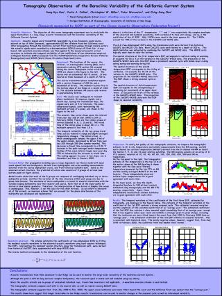
1. Tomography Observations of the Baroclinic Variability of the California Current System Sang-Kyu Han1, Curtis A. Collins1, Christopher W. Miller1, Peter Worcestor2, and Ching-Sang Chiu1 1: Naval Postgraduate School (email: skhan@nps.navy.mil, chiu@nps.navy.mil) 2: Scripps Institution of Oceanography, University of California at San Diego (Research sponsored by NOPP as part of the Ocean Acoustic Observatory FederationProject) Scientific Objective: The objective of this ocean tomography experiment was to study both the signal fluctuations in a long-range acoustic transmission and the baroclinic variability of the California Current System. Approach: Acoustic signals were transmitted repeatedly by a low-frequency sound source moored on top of Hoke Seamount, approximately 600 km offshore from the California coast. After propagating through the California Current Front and then upslope through inshore waters, the acoustic signals were recorded by a decommissioned SOSUS array off Point Sur. A ray-based, full-waveform inversion scheme was then applied to the measured acoustic arrival structure to estimate the temporal variability of the coefficients of two-dimensional empirical orthogonal functions (EOFs) analyzed from the CalCOFI(California Cooperative Oceanic Fisheries Investigations)and WOCE (World Ocean Circulation Experiment)data. where ti is the time of the ith transmission, and are respectively the complex envelopes of the observed and modeled waveforms, both normalized to have unit energy, and mk is the coefficient of the kth EOF. Only 3 EOFs were used in the least squares fit. The 3 EOFs account for 75% of the variance in the CalCOFI and WOCE data. The 2-D (two-dimensional) EOFs along the transmission path were derived from historical CalCOFI and WOCE CTD data. Most CalCOFI casts were limited to a depth of 500 m. This depth limitation was mitigated by combining the CalCOFI and WOCE data. The WOCE casts typically went down to near the bottom. The spatial structure of the first temperature EOF corresponds to surface cooling or warming. It accounts for 52.6 % of the variance in the CalCOFI-WOCE data. The projection of the CalCOFI-WOCE data onto this EOF shows a prominent seasonal cycle with mixed-layer cooling during spring and warming during fall. Experiment: The locations of the source, the receiver, an oceanographic mooring (M4), and a mesoscale resolving CTD section (X) occupied during the source deployment cruise in early May 1999 are shown in the figure to the left. The source was an autonomous HLF-5 source. It was moored on Hoke Seamount at a depth of 729 m. The source transmitted phase-modulated signals with a carrier frequency of 250 Hz and a bandwidth of 83 Hz. The SOSUS receiver lies on the bottom slope of Sur Ridge at a depth of 1360 m. The distance between the source and receiver is approximately 624 km. Data: The source was configured to transmit phase-modulated, M-sequence signals every fourth day. During the transmission days, the signals were sent at 4-hr intervals. The pulse-compressed signals, each representing the multipath arrivals of a pulse, are shown in the figure to the left. The acoustic time series shown spans the interval from year day 185 (4 July 1999) to 397 (1 February 2000).There are five stable groups of arrivals (labeled A, B, C, D and E). The travel time of the initial group is about 421.2 s. The multipath spread is less than 1.5 s. The temporal variability of the ray-group travel times can be related to range and depth averaged temperature changes. The initial arrival, A, which unambiguously samples the upper 3 km of the water column, decreased by 80 ms from year day 200 through 255 (the summer months). This decrease in travel time corresponds to a 0.06 C increase in the path-averaged water temperature. Cooling of the ocean interior began near year day 300 as indicated by the increase in travel time. The cooling appears to occur in two steps, one in November and then in January 2000. The spatial structure of the second temperature EOF corresponds to the titling of isotherms. It accounts for 15.3% of the variance in the CalCOFI-WOCE data. The projection of the CalCOFI-WOCE data onto this EOF shows a strong seasonal cycle as well. The spatial structure of third temperature EOF corresponds to the strengthening or weakening (or movement) of an upper-layer front. It accounts for 8.6% of the variance in the CalCOFI-WOCE data. The projection of the CalCOFI-WOCE data onto this EOF shows no seasonal variability. Comparison: To verify the quality of the tomographic estimate, we compare the tomographic estimate to (1) in situ temperature and salinity measurements from the M4 mooring, and (2) multi-channel sea surface temperature (MCSST) derived from the 5-channel AVHRR on board the NOAA-7, 9, 11 and 14 polar orbiting satellites. The M4 mooring consists of an array of 11 CTD sensors, mounted at 10, 20, 40, 60, 80, 100, 150, 200, 250, 300 and 340 m, respectively. On the top panel to the right, the tomographic estimate of the temperature in the top 10 m of the water column at the M4 location is shown together with the (low-pass filtered) temperature measured by the top CTD on M4 and the weekly averaged MCSST at the M4 location. These independently observed surface-layer temperatures are in good agreement with each other. In the lower panel, we show the depth-integrated (surface to 340 m) heat content, estimated using tomograrphy and the M4 CTD mooring, respectively. Again, these independently derived heat content estimates are in good agreement with each other. Forward Model:Our propagation modeling uses a range dependent ray-theory model with input sound speed field and bathymetry derived from hydrographic and echo sounding measurements obtained from the source deployment cruise, and from historical CalCOFI data. Same as the observed arrival structure, the predicted structure also consists of 5 groups of arrivals (see bottom panel on figure above). Model results show that each of the 5 groups are composed of overlapping individual-ray or micro-multipaths arrivals, and that the variation of the fine structure within each group are due to phase interference. The existence of micro-multipaths is a result of acoustic interactions with the variable sloping bathymetry near the receiver and source. Note that all of the eigen-paths for Arrival A have similar geometry. Therefore, the interpretation of how Arrival A samples the ocean is unambiguous. This, however, is not the case for the other Arrivals. In an effort to interpret all of the arrivals, an inversion scheme that can account for the phase interference of the multipaths was developed and implemented. Results: The temporal variations of the coefficientsof the first three EOF, estimated by tomography, are displayed in the figures below. The estimate of the temporal variations of the coefficient of the 1st EOF contains a strong seasonal cycle. This estimated seasonal variation and the amplitude of this variation match that of an “average year.” The estimated coefficient of the 2nd EOF also contains a clear seasonal signal resembling that of an average year, except that it has negative values year round and exhibits a stronger peak-to-peak change, revealing that the isotherms are more tilted toward the coast from July 1999 to February 2000 than an “average year.” The estimated coefficient of the 3rd EOF exhibits no seasonal variation. This is consistent with historical data. The mostly negative values, however, suggest that, from July 1999 to February 2000, the California Front was weaker than “normal.” Waveform Inversion: The scheme estimates the coefficients of two-dimensional EOFs by fitting the modeled acoustic waveform to the observed acoustic waveform using least squares techniques. The EOFs, representing the dominant spatial structure along the transmission path, were derived from historical CalCOFI data supplemented with deep WOCE data. The inverse method corresponds to the minimization of the cost function, • Conclusions: • Acoustic transmissions from Hoke Seamount to Sur Ridge can be used to monitor the large-scale variability of the California Current System. • Although the path is 624 km long and over complex bathymetry, the received signal is stable and well modeled using ray theory. • Since the acoustic arrivals are in groups of unresolved individual rays, travel-time inversion is not applicable. A waveform inversion scheme is used instead. • The tomographic estimate compares well with in situ moored data as well as remote-sensing MCSST data. • The tomographic estimate suggests that, from July 1999 to Feb. 2000, the upper-ocean isotherms were more titled toward the coast and the California Front was weaker than the “average year.” • The results shown here suggest that longer term Hoke-to-Sur Ridge acoustic transmissions can be used to monitor changes in the seasonal cycle as well as interannual variability.