Binomial Distributions for Calculations
Learn the conditions and calculations for binomial distributions, including probability, mean, and variance. Explore the use of normal approximations and vocabulary related to binomial settings.

Binomial Distributions for Calculations
E N D
Presentation Transcript
Lesson 6.3 Discrete Distribution Binomial
Knowledge Objectives • Describe the conditions that need to be present to have a binomial setting. • Define a binomial distribution. • Explain when it might be all right to assume a binomial setting even though the independence condition is not satisfied. • Explain what is meant by the sampling distribution of a count. • State the mathematical expression that gives the value of a binomial coefficient. Explain how to find the value of that expression. • State the mathematical expression used to calculate the value of binomial probability.
Construction Objectives • Evaluate a binomial probability by using the mathematical formula for P(X = k). • Explain the difference between binompdf(n, p, X) and binomcdf(n, p, X). • Use your calculator to help evaluate a binomial probability. • If X is B(n, p), find µx and x (that is, calculate the mean and variance of a binomial distribution). • Use a Normal approximation for a binomial distribution to solve questions involving binomial probability
Vocabulary • Binomial Setting – random variable meets binomial conditions • Trial – each repetition of an experiment • Success – one assigned result of a binomial experiment • Failure – the other result of a binomial experiment • PDF – probability distribution function; assigns a probability to each value of X • CDF – cumulative (probability) distribution function; assigns the sum of probabilities less than or equal to X • Binomial Coefficient – combination of k success in n trials • Factorial – n! is n (n-1) (n-2) … 2 1
Criteria for a Binomial Setting A random variable is said to be a binomial provided: • The experiment is performed a fixed number of times. Each repetition is called a trial. • The trials are independent • For each trial there are two mutually exclusive (disjoint) outcomes: success or failure • The probability of success is the same for each trial of the experiment Most important skill for using binomial distributions is the ability to recognize situations to which they do and don’t apply
Example 1a Does this setting fit a binomial distribution? Explain • NFL kicker has made 80% of his field goal attempts in the past. This season he attempts 20 field goals. The attempts differ widely in distance, angle, wind and so on. Probably not binomial – probability of success would not be constant
Example 1b Does this setting fit a binomial distribution? Explain • NBA player has made 80% of his foul shots in the past. This season he takes 150 free throws. Basketball free throws are always attempted from 15 ft away with no interference from other players. Probably binomial – probability of success would be constant
Binomial Notation There are n independent trials of the experiment Let p denote the probability of success and then 1 – p is the probability of failure Let x denote the number of successes in n independent trials of the experiment. So 0 ≤ x ≤ n Determining probabilities: With your calculator, go to the Distribution menu: 2nd DISTR A yields 2nd DISTR B yields binompdf(n,p,x) binomcdf(n,p,x) Some Books have binomial tables, ours does not
Binomial PDF vs CDF • Abbreviation for binomial distribution is B(n,p) • A binomial pdf function gives the probability of a random variable equaling a particular value, i.e., P(x=2) • A binomial cdf function gives the probability of a random variable equaling that value or less , i.e., P(x ≤ 2) • P(x ≤ 2) = P(x=0) + P(x=1) + P(x=2)
English Phrases P(x ≤ A) = cdf (A) P(x = A) = pdf (A) P(X) ∑P(x) = 1 Cumulative probability or cdf P(x ≤ A) P(x > A) = 1 – P(x ≤ A) Values of Discrete Variable, X X=A
Binomial PDF The probability of obtaining x successes in n independent trials of a binomial experiment, where the probability of success is p, is given by: P(x) = nCx px (1 – p)n-x, x = 0, 1, 2, 3, …, n nCx is also called a binomial coefficient and is defined by combination of n items taken x at a time or where n! is n (n-1) (n-2) … 2 1 n n! = -------------- k k! (n – k)!
TI-83 Binomial Support • For P(X = k) using the calculator: 2nd DISTR binompdf(n,p,k) • For P(k ≤ X) using the calculator: 2nd DISTR binomcdf(n,p,k) • For P(X ≥ k) use 1 – P(k < X) = 1 – P(k-1 ≤ X)
Example 2 In the “Pepsi Challenge” a random sample of 20 subjects are asked to try two unmarked cups of pop (Pepsi and Coke) and choose which one they prefer. If preference is based solely on chance what is the probability that: a) 6 will prefer Pepsi? b) 12 will prefer Coke? P(d=P) = 0.5 P(x) = nCx px(1-p)n-x P(x=6 [p=0.5, n=20]) = 20C6 (0.5)6(1- 0.5)20-6 = 20C6 (0.5)6(0.5)14 = 0.037 P(x=12 [p=0.5, n=20]) = 20C12 (0.5)12(1- 0.5)20-12 = 20C12 (0.5)12(0.5)8 = 0.1201
Example 2 cont P(d=P) = 0.5 P(x) = nCx px(1-p)n-x c) at least 15 will prefer Pepsi? d) at most 8 will prefer Coke? P(at least 15) = P(15) + P(16) + P(17) + P(18) + P(19) + P(20) Use cumulative PDF on calculator P(X ≥ 15) = 1 – P(X ≤ 14) = 1 – 0.9793 = 0.0207 P(at most 8) = P(0) + P(1) + P(2) + … + P(6) + P(7) + P(8) Use cumulative PDF on calculator P(X ≤ 8) = 0.2517
Example 3 A certain medical test is known to detect 90% of the people who are afflicted with disease Y. If 15 people with the disease are administered the test what is the probability that the test will show that: a) all 15 have the disease? b) at least 13 people have the disease? P(x) = nCx px(1-p)n-x P(Y) = 0.9 P(x=15 [p=0.9, n=15]) = 15C15 (0.9)15(1- 0.9)15-15 = 15C15 (0.9)15(0.1)0 = 0.20589 P(at least 13) = P(13) + P(14) + P(15) Use cumulative PDF on calculator P(X ≥ 13) = 1 – P(X ≤ 12) = 1 – 0.1841 = 0.8159
Example 3 cont P(Y) = 0.9 P(x) = nCx px(1-p)n-x c) 8 have the disease? P(x=8 [p=0.9, n=15]) = 15C8 (0.9)8(1- 0.9)15-8 = 15C8 (0.9)8(0.1)7 = 0.000277
Summary and Homework • Summary • Binomial experiments have 4 specific criteria that must be met • Fixed number of trials • Independent • Two mutually exclusive outcomes • Probability of success is constant • Calculator has pdf and cdf functions • Homework • pg

