Download
1 / 60
600 likes | 728 Vues
Pietro FRE’. CAPRI COFIN MEETING 2003. Cosmological Backgrounds of String Theory, Solvable Algebras and Oxidation. A fully algebraic machinery to generate, classify and interpret Supergravity solutions. E 8. D=10 SUGRA. D=10 SUGRA. dimensional oxidation. E 8 maps D=10 backgrounds

E N D
Pietro FRE’ CAPRI COFIN MEETING 2003 Cosmological Backgrounds of String Theory, Solvable Algebras and Oxidation A fully algebraic machinery to generate, classify and interpret Supergravity solutions
E8 D=10 SUGRA D=10 SUGRA dimensional oxidation E8 mapsD=10 backgrounds into D=10 backgrounds dimensional reduction Not unique: classified by different embeddings E8 D=3 sigma model D=3 sigma model Field eq.s reduce to Geodesic equations on Solutions are classified by abstract subalgebras Since all fields are chosen to depend only on one coordinate, t = time, then we can just reduce everything to D=3, D=2 or D=1. In these dimensions every degree of freedom (bosonic) is a scalar THE MAIN IDEA NOMIZU OPERATOR SOLVABLE ALGEBRA COMPENSATOR METHOD TOINTEGRATE GEODESIC EQUATIONS
What follows next is a report on work both published and to be published • Based on a collaboration by: • P. F. , F. Gargiulo, K. Rulik (Torino, Italy) • M. Trigiante (Utrecht, The Nederlands) • V. Gili (Pavia, Italy) • A. Sorin (Dubna, Russian Federation)
Maximal Susy implies Er+1 series Scalar fields are associated with positive roots or Cartan generators
How to build the solvable algebra Given the Real form of the algebra U, for each positive root there is an appropriate step operator belonging to such a real form
ST algebra W is a nilpotent algebra including no Cartan The type IIA chain of subalgebras
U duality in D=10 The Type IIB chain of subalgebras
With target manifold If we compactify down to D=3we have E8(8) Indeed the bosonic Lagrangian of both Type IIA and Type IIB reduces to the gravity coupled sigma model
+ Spinor weight Painting the Dynkin diagram = constructing a suitable basis of simple roots Type II B painting
- A second painting possibility Type IIA painting
SO(7,7) Dynkin diagram Neveu Schwarz sector Surgery on Dynkin diagram - Spinor weight = Ramond Ramond sector
String Theory understanding of the algebraic decomposition Parametrizes both metrics Gijand B-fields Bij on the Torus Internal dilaton B-field Metric moduli space
Dilaton and radii are in the CSA The extra dimensions are compactified on circles of various radii
THE FIELD EQUATIONS OF 10d SUPERGRAVITY AS GEODESIC EQUATIONS ON
Decoupling 3D gravity continues... K is a constant by means of the field equations of scalar fields.
The matter field equations are geodesic equations in the target manifold U/H • Geodesics are fixed by initial conditions • The starting point • The direction of the initial tangent vector • SinceU/H is a homogeneous space all initial points are equivalent • Initial tangent vectors span a representation ofHand by means of H transformations can be reduced to normal form. The orbits of geodesics contain as many parameters as that normal form!!!
Orthogonal decomposition Non orthogonal decomposition The orbits of geodesics are parametrized by as many parameters as the rank of U Indeed we have the following identification of the representationK to which the tangent vectors belong:
and since We can conclude that any tangent vector can be brought to have only CSA components by means of H transformations The cosmological solutions in D=10 are therefore parametrized by 8 essential parameters. They can be obtained from an 8 parameter generating solution of the sigma model by means of SO(16) rotations. The essential point is to study these solutions and their oxidations
and turn them to the anholonomic basis • The strategy to solve the differential equations consists now of two steps: • First solve the first order differential system for the tangent vectors • Then solve for the coset representative that reproduces such tangent vectors
Summarizing: • If we are interested in time dependent backgrounds of supergravity/superstrings we dimensionally reduce to D=3 • In D=3 gravity can be decoupled and we just study a sigma model on U/H • Field equations of the sigma model reduce to geodesics equations. The Manifold of orbits is parametrized by the dual of the CSA. • Geodesic equations are solved in two steps. • First one solves equations for the tangent vectors. They are defined by the Nomizu connection. • Secondly one finds the coset representative • Finally we oxide the sigma model solution to D=10, namely we embed the effective Lie algebra used to find the solution into E8. Note that, in general there are several ways to oxide, since there are several, non equivalent embeddings.
The H compensator method THIS A SYSTEM OF DIFFERENTIAL EQUATIONS FOR THE H-PARAMETERS
The Compensator Equations Solving the differential system for the compensators is fully equivalent to solving the original system of equations for the tangent vectors The compensator system however is triangular and can be integrated by quadratures For instance for the A2 system these equations are
The solution contains threeintegration constants. Together with the two constanst of the generating solution this makes five. We had five equations of the first order. Hence we have the general integral !! Explicit Integration of the compensator equations for the A2 system
AS AN EXAMPLE WE DISCUSSTHE SIMPLEST SOLUTION (One rotation only )and SOME OF ITS OXIDATIONS
Explicit solution for the tangent vectorsand the scalar fields after one rotation
Next we consider the equations for the scalar fields: The equations for the scalar fields can always be integrated because they are already reduced to quadratures. The form of the vielbein is obtained by calculating the left invariant 1—form from the coset representative: The order is crucial: from left to right, decreasing grade. This makes exact comparison with supergravity
This is the final solution for the scalar fields, namely the parameters in the Solvable Lie algebra representation This solution can be OXIDED in many different ways to a complete solution of D=10 Type IIA or Type IIB supergravity. This depends on the various ways of embedding the A2 Lie algebra into the E8 Lie algebra. The physical meaning of the various oxidations is very much different, but they are related by HIDDEN SYMMETRY transformations.
Type II B Action and Field equations in D=10 Where the field strengths are: Chern Simons term Note that the Chern Simons term couples the RR fields to the NS fields !!
PROBLEM: Where the physical interpretation of the subalgebras and the correspondence with roots is There are several inequivalent ways, due to the following graded structure of the Solvable Lie algebra of E8
Choosing an example of type 4 embedding • Physically this example corresponds to a superposition of three extended objects: • An euclidean NS 1-brane in directions 34 or NS5 in directions 1256789 • An euclidean D1-brane in directions 89 or D5 in directions 1234567 • An euclidean D3-brane in directions 3489
In this context, the two parameters of the A2 generating solution of the following interpretation: If we oxide our particular solution... Note that B34 = 0 ; C89= 0 since in our particular solution the tangent vector fields associated with the roots a1,2 are zero. Yet we have also the second Cartan swtiched on and this remembers that the system contains not only the D3 brane but also the 5-branes. This memory occurs through the behaviour of the dilaton field which is not constant rather it has a non trivial evolution. The rolling of the dilaton introduces a distinction among the directions pertaining to the D3 brane which have now different evolutions.
The effective field equations for this oxidation For our choice of oxidation the field equations of type IIB supergravity reduce to 5 brane contribution to the stress energy tensor D3 brane contribution to the stress energy tensor and one can easily check that they are explicitly satisfied by use of the A2 model solution with the chosen identifications
Explicit Oxidation: The Metricand the Ricci tensor Non vanishing Components of Ricci
Plots of the Radii for the case with We observe the phenomenon of cosmological billiard of Damour, Nicolai, Henneaux
P in 567 P in 89 P in 12 P in 34 Energy density and equations of state