Ultrasound
Ultrasound . Introduction SRAD Filter Wiener Filter SNR comparison Diagnosis using ANN. Introduction. History : Sound technology was utilized in the early nineteenth century for measuring distances underwater.

Ultrasound
E N D
Presentation Transcript
Ultrasound Introduction SRAD Filter Wiener Filter SNR comparison Diagnosis using ANN
Introduction • History : • Sound technology was utilized in the early nineteenth century for measuring distances underwater. • In 1958, Donald and his colleagues published the most important paper in biomedical ultrasound. • Definition : Waves of higher frequency than audible sound waves. It is approximately 20 KHz.
Introduction • Ultrasonography : • It is an ultrasound-based diagnostic imaging technique used to visualize body structures including muscles, joints, vessels and internal organs. • The frequencies of sound waves used in ultrasonography are between about (1 and 15) MHz.
Introduction • How are images acquired for ultrasound ?
Introduction Advantages Disadvantages • Image muscle, soft tissue, and bone surfaces very well. • Show the structure of organs. • No known long-term side effects. • Equipment is widely available & flexible. • Relatively inexpensive compared to other modes of investigation. • Sonographic devices have trouble penetrating bone. • The depth of penetration of ultrasound may be limited depending on the frequency of imaging. • Operator-dependent.
Introduction • Ultrasound Vs X-Ray :
DespeckleFiltering Images acquired by ultrasound are corrupted by speckles. • Speckle noise : Here the speckle phenomenon results from the constructive-destructive interference of the coherent ultrasound pulses back scattered from the tissues. • We have 2 types of despeckle filters : • SRAD Filter • Wiener Filter
SRAD Filter • SRAD : Speckle Reducing Anisotropic Diffusion. • SRAD : non-linear technique for multiplicative noise reduction and image enhancement. • SRAD concept : 1. making intra-region smoothing (in homogeneous regions) and preserve edges. “q” (coefficient of variation) controls this variation. 2. using PDE approach for speckle removal.
SRAD Filter • “q” (coefficient of variation) : achieves a balance between : 1. smoothing in homogeneous regions (average-like filtering). 2.preserving edges (identity filtering). • How is this balance achieved ? using thresholds to alter the performance between average-like filtering (in homogeneous regions) & identity filtering (at edges).
SRAD Filter • Why SRAD ? 1. SRAD is not sensitive to the size of filter window (as in conventional despeckle filters). 2. SRAD doesn’t utilize hard thresholds , as hard thresholds lead to blotching the images. 3. SRAD not only preserves edges but also enhance edges by inhibiting the diffusion process near edges.
SRAD Filter • SRAD Performance : speckle removal is achived using SRAD PDE approach : Where : c(q) : diffusion coefficient. • Etymology :c(q) is anisotropic (direction variant properties) so , this method of removing speckle noise is called Speckle Reducing Anisotropic Diffusion or SRAD.
SRAD Filter • Solution of SRAD PDE :(discretization) • t = n ∆t , n = 0 , 1 , 2 , ………. , ∆t is iteration step size. x = ih , i = 0 , 1 , 2 , …….. , M-1. y = jh , j = 0 , 1 , 2 , ………, N-1. • By this way of discretization , then MhхNh is the size of the image. Let according to the previous assumptions will be : = I (ih , jh , n ∆t ).
SRAD Filter • First Stage : calculate the . • Second Stage : calculate diffusion coefficient c(q). • Third Stage : calculate the divergence of which is • Finally : we can substitue using the previous 3 stages to reach the final result which is : = + • This iterative relation shows that we need much computation time , and also shows how to control the diffusion process.
SRAD Filter Flow Chart : start Applying SRAD filter on image Close figures & Clear variables Reading the image Wait for processing and loading according to the no. of iterations Choose a rect. of the desired part of image Getting O/P filtered image End
SNR Calculation • We can use the following equation to get the SNR value :
SNR Calculation start Flow Chart : no yes Get no. of rows & columns M×N Set initial value for numerator Loop for numerator Loop finished ? Wait for summation of elements
SNR Calculation no yes Set initial value for denominator Loop for denominator Loop finished ? Wait for summation of elements SNR =numerator / denominator End
Results • Ultrasound on fetus : (SNR = 23.658)
Results • SpinaPifida : (SNR = 17.868)
Results • Hydrocephalus : (SNR = 35.424)
Results • Kidney dysplasia : (SNR =67.094)
Results • Atrialseptal defect : (SNR =53.862)
Results • Fatty liver : (SNR =53.767)
Results • Diaphragmatic hernia : (SNR =26.468)
Results • Cerebral Palsy : (SNR =25.579)
Conclusion • SRAD filter is a good way that removes speckle noise from ultrasound images efficiently and makes intra-region smoothing (in homogeneous regions) and preserve edges. • SRAD takes long computation time for iterations & has relatively lower SNR value.
WienerFilter • Proposed by “Norbert Wiener” in 1940s. • Purpose : filter out speckle noise that has corrupted the image, based on statistical approach. • Method : Its purpose is to reduce the amount of noise present in the image by comparison with an estimation of the desired noiseless image. • It is characterized by : The optimal estimator (in the sense of Mean Squared Error (MSE)) for stationary Gaussian process.
WienerFilter • Equation: • Duo to : so, we can’t use Wiener filter for true images. We can use Local Adaptive Wiener Filter
LocalAdaptiveWienerFilter • Why Local : Because image isn’t stationary as the assuumption of Wiener filter. But, we can say Locally stationary (samples of image are stationary and samples are nonstatinary). That is done using {LLMMSE} • Why Adaptive : Becauseit is used to determine the nonstationary weights that are in the image due to its abrupt changes of image intensities. That is done using {AWA} function. In general we can say that ,it can smooth image and leave edges with out change.
LocalAdaptiveWienerFilter Consider the filtering of images corrupted by image independent zero-mean white Gaussian noise. The problem can be modeled as : Where : • y(i, j) : the noisy measurement. • x(i, j) : the noise free image. • n(i,j) : additive Gaussian noise. Where : N : the number of elements in x(i,j).
LocalAdaptiveWienerFilter • When x(i, j) and n(i, j) are stationary Gaussian processes Where : • σ²x : the variance of image . • μx : the mean of image. • μn : the mean of noise and assumed to be zero. Here we assume that we know the mean and the variance of the image from the characteristics of stationary Gaussian process .
LocalAdaptiveWienerFilter By tacking uniform moving average window of size (2r + 1) × (2r + 1) We can get Local Mean and Local Variance as shown: Till now , the resulting denoised image is poor and looks noisy. To blur the mean and increase the variance near edges,We use weighted form
LocalAdaptiveWienerFilter • Where : Where The parameters of this weighting function are: • α> 0 • ε = 2.5 σn • α ε² ≥ 1
LocalAdaptiveWienerFilter Flow Chart : start Applying Wiener filter on image Close figures & Clear variables Reading the image Getting O/P filtered image Calculate SNR Convert Uint8 to Double End
Results • Ultrasound on fetus : (SNR = 28.371)
Results • Spina Bifida : (SNR = 28.566)
Results • Hydrocephalus : (SNR = 45.566)
Results • Kidney dysplasia : (SNR = 78.592)
Results • AtrialSeptal Defect : (SNR =65.162)
Results • Fatty Liver : (SNR =62.416)
Results • Diaphragmatic hernia : (SNR =30.373)
Results • Cerebral Palsy : (SNR =43.080)
SRAD Vs Wiener • In Wiener , we reduce the amount of noise present in the image by comparison with an estimation of the desired noiseless image. But no comparison in SRAD. • In SRAD , we need much computation time as a result of many iteration loops. But in Wiener we don’t. • Wiener is linear and SRAD is non-linear. • SNR of image filtered by SRAD is a bit less than Wiener.
Conclusion The Local Adaptive Wiener Filter is a good mean to reduce the amount of speckles noise in the images. It has a higher SNR than SRADwhich means a higher quality of image. No long computation time.
Diagnosis using ANN ANN is divided into TWO stages: • The first one is TRAINING. • The second one RECALLING. • Training: Is to learn the network the image and its number with its disease name. • Recalling: Is to give the number of the image to the network and it will give you the image with its disease name.
Results • Training:
Results • Recalling: • If you Press 1 :