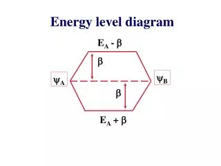
Energy level diagram
480 likes | 734 Vues
. B. A. . E A + . Energy level diagram. E A - . Linear combination of atomic orbitals. Rules for linear combination. 1. Atomic orbitals must be roughly of the same energy.

Energy level diagram
E N D
Presentation Transcript
B A EA + Energy level diagram EA -
Linear combination of atomic orbitals Rules for linear combination 1. Atomic orbitals must be roughly of the same energy. 2. The orbital must overlap one another as much as possible- atoms must be close enough for effective overlap. 3. In order to produce bonding and antibonding MOs, either the symmetry of two atomic orbital must remain unchanged when rotated about the internuclear line or both atomic orbitals must change symmetry in identical manner.
Rules for the use of MOs * When two AOs mix, two MOs will be produced * Each orbital can have a total of two electrons (Pauli principle) * Lowest energy orbitals are filled first (Aufbau principle) * Unpaired electrons have parallel spin (Hund’s rule) Bond order = ½ (bonding electrons – antibonding electrons)
Linear Combination of Atomic Orbitals (LCAO) The wave function for the molecular orbitals can be approximated by taking linear combinations of atomic orbitals. A B c – extent to which each AO contributes to the MO AB = N(cA A + cBB) 2AB = (cA2A2 + 2cAcB A B + cB2 B 2) Overlap integral Probability density
Amplitudes of wave functions added Constructive interference g bonding cA = cB = 1 g = N [A + B]
2AB = (cA2A2 + 2cAcB A B + cB2 B 2) density between atoms electron density on original atoms,
The accumulation of electron density between the nuclei put the electron in a position where it interacts strongly with both nuclei. Nuclei are shielded from each other The energy of the molecule is lower
node + - u cA = +1, cB = -1 antibonding u = N [A - B] Amplitudes of wave functions subtracted. Destructive interference Nodal plane perpendicular to the H-H bond axis (en density = 0) Energy of the en in this orbital is higher. A-B
The electron is excluded from internuclear region destabilizing Antibonding
Molecular potential energy curve shows the variation of the molecular energy with internuclear separation.
Looking at the Energy Profile • Bonding orbital • called 1s orbital • s electron • The energy of 1s orbital decreases as R decreases • However at small separation, repulsion becomes large • There is a minimum in potential energy curve
H2 11.4 eV 109 nm LCAO of n A.O n M.O. Location of Bonding orbital 4.5 eV
The overlap integral • The extent to which two atomic orbitals on different atom overlaps : the overlap integral
S > 0 Bonding S < 0 anti Bond strength depends on the degree of overlap S = 0 nonbonding
Homonuclear Diatomics • MOs may be classified according to: • (i) Their symmetry around the molecular axis. • (ii) Their bonding and antibonding character. • 1s 1s* 2s 2s* 2p y(2p) = z(2p) y*(2p) z*(2p)2p*.
B g- identical under inversion A u- not identical
Place labels g or u in this diagram s*u p*g pu sg
First period diatomic molecules H H2 H u* Energy 1s 1s g 1s2 Bond order: 1 Bond order = ½ (bonding electrons – antibonding electrons)
He He2 He u* Energy 1s 1s g Diatomic molecules: The bonding in He2 1s2, *1s2 Bond order: 0 Molecular Orbital theory is powerful because it allows us to predict whether molecules should exist or not and it gives us a clear picture of the of the electronic structure of any hypothetical molecule that we can imagine.
Second period diatomic molecules 1s2, *1s2, 2s2 Li Li2 Li Bond order: 1 2u* 2s 2s 2g Energy 1u* 1s 1s 1g
Diatomic molecules: Homonuclear Molecules of the Second Period Be Be2 Be 2u* 1s2, *1s2, 2s2, *2s2 2s 2s 2g Energy Bond order: 0 1u* 1s 1s 1g
MO diagram for B2 3u* 1g* 1u 3g 2u* 2g Diamagnetic??
Li : 200 kJ/mol F: 2500 kJ/mol
Same symmetry, energy mix- the one with higher energy moves higher and the one with lower energy moves lower
MO diagram for B2 B B B2 3u* 3u* 1g* 1g* 2p (px,py) 1u 2p 3g 3g LUMO HOMO 1u 2u* 2u* 2s 2s 2g 2g Paramagnetic
1g 1g 1u 1u 1g 1g C2 Diamagnetic X Paramagnetic ?
1g 1g 1u 1u 1g 1g General MO diagrams O2 and F2 Li2 to N2
Filling bonding orbitals Filling antibonding orbitals Bond lengths in diatomic molecules
Summary From a basis set of N atomic orbitals, N molecular orbitals are constructed. In Period 2, N=8. The eight orbitals can be classified by symmetry into two sets: 4 and 4 orbitals. The four orbitals from one doubly degenerate pair of bonding orbitals and one doubly degenerate pair of antibonding orbitals. The four orbitals span a range of energies, one being strongly bonding and another strongly antibonding, with the remaining two orbitals lying between these extremes. To establish the actual location of the energy levels, it is necessary to use absorption spectroscopy or photoelectron spectroscopy.
Heteronuclear Diatomics…. • The energy level diagram is not symmetrical. • The bonding MOs are closer to the atomic orbitals which are lower in energy. • The antibonding MOs are closer to those higher in energy. c – extent to which each atomic orbitals contribute to MO If cAcB the MO is composed principally of A
HF 1s 1 2s, 2p 7 =c1 H1s + c2 F2s + c3 F2pz Largely nonbonding 2px and 2py 12 2214 Polar