SOLVING INVERSE ODE USING BEZIER FUNCTIONS
SOLVING INVERSE ODE USING BEZIER FUNCTIONS. P. Venkataraman. The Inverse ODE Problem. The inverse problem in this paper is very primitive: find the differential equation and the boundary conditions if the discrete solution is known everywhere. OR.


SOLVING INVERSE ODE USING BEZIER FUNCTIONS
E N D
Presentation Transcript
SOLVING INVERSE ODE USING BEZIER FUNCTIONS P. Venkataraman
The Inverse ODE Problem • The inverse problem in this paper is very primitive: • find the differential equation and the boundary conditions • if the discrete solutionis known everywhere OR If [xi, yi], i = 1,2, .. p is known as the solution to Then find f(D) and y0 f(D) may be a linear or a nonlinear operator The ODE is homogenous after all the forward or the direct boundary value problem is the determination of the solution everywhere if the differential equation is known and the boundary conditions are given
Current Types of Inverse Problems Inverse problems investigated today belong to one of three types (i) Identifying parameters in a known form of the differential equation based on the particular knowledge domain (ii) Identifying boundary conditions at points that are not easily accessible using excess data at other points (iii) establishing some functions on the domain that are tied to the known form of the differential equations Most of the investigations today use some form of element discretization in two dimensional domain
The Solution Process • The procedure involves two steps: • A “best” Bezier function is fitted to the data • This function, which is also the solution to the ODE, will satisfy the differential equation and identify the boundary condition • The specific form of the differential equation is determined • This form is established from a generic representation of the ODE using a set of exponent and coefficient values
Why a Bezier Function? Bezier functions are parametric curves based on Bernstein polynomial basis functions • Bezier functions can provide explicit solutions to the forward boundary value problem very effectively • The author’s papers in previous CIE conferences have shown Bezier functions can solve linear or nonlinear, single or multi variable, ordinary or partial differential equations, with initial and/or boundary values “the Bernstein polynomial approximation to a continuous function mimics the gross features of the function remarkably well” - Gordon and Riesenfeld As the order of the polynomial is increased, this approximation converges uniformly to the function and its derivatives where they exist The Bezier curve delivers, at the minimum, the same smoothness as the primitive function it is trying to emulate
What is a Bezier Function ? A Bezier function is a Bezier curve that behaves like a function The Bezier curve is defined using a parameter Instead of y=f(x); both x and y depend on the same parameter value; x = x(p) and y = y(p) p : parameter Bernstein basis Number of vertices: 5 Order of the function : 4
Matrix Description of Bezier Function (2D) This allows the use of Array Processing for shorter computer time
Step 1:The Best Bezier Function to fit the Data For a selected order of the Bezier function (n) Given a set of (m) vector data ya,i, or [Y], find the coefficient matrix, [B] so that the corresponding data set yb,i , [YB ] produces the least sum of the squared error Minimize FOC: Once the coefficient matrix is known, all other information, including the derivatives can be generated using array processing The best m is determined by the lowest value of E This is Step 1 of the solution process
Step 2:The Generic Form of ODE Many 3rd order ODE generic forms are used in the paper. For example Linear Generic Form • There are two types of unknowns: • the exponents of the derivatives • the coefficients multiplying the terms • The exponents are expected to be integers • The coefficients are unrestricted • The function and its derivatives are known quantities after Step 1 Nonlinear Generic Form
Establishing the Unknowns A Least Squared Error Technique is used to determine the unknowns N: the number of data points This is the objective for linear constant coefficient form A similar one can be used for the generic nonlinear form A continuous application of standard optimization technique was unsuccessful because the exponents were not integers A mixed integer (exponents) – continuous (coefficients) approach was also unsuccessful because the solution will determine trivial values Solution was only possible through discrete programming
Discrete Programming Used in The Paper Two procedures are considered in this paper • 1. Exhaustive Enumeration • all of the values for the unknowns are considered in combination before the optimum is determined • Simple Heuristic Programming • simple heuristic exhaustive enumeration over predetermined number of cycles (1 billion) Discrete Programming is incredibly time extensive For the linear constant coefficient form, allowing 3 values for each unknown required 1.0*105 cpu seconds on a Linux Opteron running MATLAB 2007a
Example 1 (Step 1) Best order of Fit (based on y-data) : 14 Number of data points: 200 Sum of Absolute Error (y): 7.27217e-005 Sum of Squared Error (y): 3.96250e-011 Average Error (y): 3.63608e-007 Sum of Absolute Error (x): 4.56362e-007 Sum of Squared Error (x): 2.05982e-015 Average Error (x): 2.28181e-009 The original data is discrete x-y data The derivatives are those predicted for the data
Example 1 (Step 2) The exponents and coefficients are drawn from the set of three except for h1 that will belong to a set of 9 values Solution : Exhaustive Enumeration The solution for the exponents: a1 = 0, a2 = 1, a3 = 1, a4 = 1, b1 = 1, b2 = 0, b3 = 0, c1 = 1, c2 = 0, d1 = 1. The solution for the coefficients: e1 = 1, e2 = 1, e3 = 1, f1 = 0, f2 = 0, f3 = 1, g1 = 0, g2 = 1, g3 = 0, h1 = -0.25 h2 = 0, h3 = 1. The differential equation This was the same differential equation used to generate the discrete data
Example 2 (Step 1) Best order of Fit (based on y-data): 12 No. of data points: 101 Sum of Absolute Error (y): 8.90327e-005 Sum of Squared Error (y): 1.51515e-010 Average Error (y): 8.81512e-007 Sum of Absolute Error (x): 1.23819e-008 Sum of Squared Error (x): 2.26533e-018 Average Error (x): 1.22593e-010 The discrete data is created by numerical integration using derivative information The Bezier data approximates the derivative nicely
Example 2 (Step 2) A constant nonlinear generic form is used (to reduce time of computation) Solution : Exhaustive Enumeration The solution for the exponents: a1 = 1, a2 = 1, a3 = 2, a4 = 0, b1 = 2, b2 = 2, b3 = 1, c1 = 0, c2 = 0, d1 = 0 The solution for the coefficients: e1 = 1, e2 = 0.5, e3 = 0.5, e4 = 0.5 The differential equation This is the Blasius equation used to generate data
Conclusions and Future Work A two-phased approach is used to identify the ODE from discrete solution data through discrete programming using LSQ criterion 1. Identify the best Bezier function that fits the data This will provide information on the boundary conditions 2. Find the exponents and coefficients of appropriate generic ODE This will identify the particular ODE The computation time is a serious issue for a broader range of values. Global optimization techniques may provide a relief Extension to coupled ODE single and coupled PDE non smooth data are planned for the future