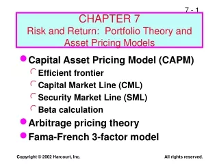
Chapter 7 An Introduction to Asset Pricing Models
530 likes | 767 Vues
Chapter 7 An Introduction to Asset Pricing Models. Recall: The Portfolio Management Process. Policy statement (road map)- Focus: Investor ’ s short-term and long-term needs, familiarity with capital market history, and expectations

Chapter 7 An Introduction to Asset Pricing Models
E N D
Presentation Transcript
Chapter 7 An Introduction to Asset Pricing Models
Recall:The Portfolio Management Process • Policy statement (road map)- Focus: Investor’s short-term and long-term needs, familiarity with capital market history, and expectations 2. Examine current and projected financial, economic, political, and social conditions - Focus: Short-term and intermediate-term expected conditions to use in constructing a specific portfolio 3. Implement the plan by constructing the portfolio - Focus: Meet the investor’s needs at the minimum risk levels 4. Feedback loop: Monitor and update investor needs, environmental conditions, portfolio performance Exhibit 2.2
Background for Capital Market Theory A. Capital Market Theory: assumptions 1. All investors are Markowitz efficient investors who want to target points on the efficient frontier. • The exact location on the efficient frontier and the specific portfolio selected will depend on the individual investor’s utility function.
2. Investors can borrow or lend any amount of money at the risk-free rate of return (RFR). • It is always possible to lend money at the nominal risk-free rate by buying risk-free securities. • It is not always possible to borrow at this risk-free rate, but later we will see that a higher borrowing rate does not change the general results.
3. All investors have homogeneous expectations; that is, they estimate identical probability distributions for future rates of return.
4. All investors have the same one-period time horizon such as one-month, six months, or one year. • A difference in the time horizon would require investors to derive risk measures and risk-free assets that are consistent with their time horizons.
5. All investments are infinitely divisible, which means that it is possible to buy or sell fractional shares of any asset or portfolio.
6. There are no taxes or transaction costs involved in buying or selling assets. • This is a reasonable assumption in many instances. Neither pension funds nor religious groups have to pay taxes, and the transaction costs for most financial institutions are less than 1 percent on most financial instruments.
7. There is no inflation or any change in interest rates, or inflation is fully anticipated.
8. Capital markets are in equilibrium. • This means that we begin with all investments properly priced in line with their risk levels.
Background for Capital Market Theory B. Risk-Free Asset • An asset with zero standard deviation • Zero correlation with all other risky assets • Provides the risk-free rate of return (RFR) • Will lie on the vertical axis of a return-risk graph
Because the returns for the risk free asset (suppose “i”=“RF”) are certain Thus Ri = E(Ri), and Ri - E(Ri) = 0 Consequently, the covariance of the risk-free asset with any risky asset or portfolio will always equal zero.
Combining a risk-free asset with a risky portfolio Expected return computation: w: weight
Risk computation: The expected variance for a two-asset portfolio is When asset 1 is a risk-free asset:
Given the variance formula the standard deviation is
Exhibit 7.1 D M C B A RFR Portfolio Possibilities Combining the Risk-Free Asset and Risky Portfolios
Risk-Return Possibilities with Leverage To attain a higher expected return than is available at point M: • Either invest along the efficient frontier beyond point M, such as point D. • Or, add leverage to the portfolio by borrowing money at the risk-free rate and investing in the risky portfolio at point M.
Exhibit 7.1 D M C B A RFR
Exhibit 7.2 CML Borrowing Lending M RFR
The Market Portfolio • Portfolio M • lies at the point of tangency • has the highest portfolio possibility line • Everybody will want to invest in Portfolio M, then borrow or lend at risk-free rate. (The combination will lie on CML.) • M must include all risky assets
The Market Portfolio • Because it contains all risky assets, it is a completely diversified portfolio. • All the unique risk of individual assets (unsystematic risk) is diversified away.
Systematic Risk • Only systematic risk remains in the market portfolio. • Systematic risk is the variability in all risky assets caused by macroeconomic variables. • Systematic risk can be measured by the standard deviation of returns of the market portfolio.
Exhibit 7.3 Standard Deviation of Return Unsystematic (diversifiable) Risk Total Risk Systematic Risk Number of Stocks in the Portfolio Standard Deviation of the Market Portfolio (systematic risk)
The CML and the Separation Theorem • The CML leads all investors to invest in the M portfolio. • Individual investors should differ in position on the CML depending on risk preferences.
How an investor gets to a point on the CML is based on financing decisions. • Risk lovers might borrow funds at the RFR and invest everything in the market portfolio. • Risk averse investors will lend part of the portfolio at the risk-free rate and invest the remainder in the market portfolio.
Optimal Portfolio Choices on the CML Exhibit 7.4
A Risk Measure for the CML • Covariancewith the M portfolio is the systematic risk of an asset. • Because all individual risky assets are part of the M portfolio, an asset return in relation to the M return can be shown as: where: Rit = return for asset i during period t ai = constant term for asset i bi = slope coefficient for asset i RMt = return for the M portfolio during period t ε= random error term
The Security Market Line (SML) • The relevant risk measure for an individual risky asset is its covariance with the market portfolio (Covi,m) • The return for the market portfolio should be consistent with its own risk:
Exhibit 7.5 SML Market Portfolio RFR Graph of Security Market Line (SML)
The Security Market Line (SML) The equation for the risk-return line is
Exhibit 7.6 SML RFR Graph of SML with Normalized Systematic Risk Negative Beta
Determining the Expected Rate of Return for a Risky Asset Assume: RFR = 6% (0.06) RM = 12% (0.12) Implied market risk premium = 6% (0.06) E(RA) = 0.06 + 0.70 (0.12-0.06) = 0.102 = 10.2% E(RB) = 0.06 + 1.00 (0.12-0.06) = 0.120 = 12.0% E(RC) = 0.06 + 1.15 (0.12-0.06) = 0.129 = 12.9% E(RD) = 0.06 + 1.40 (0.12-0.06) = 0.144 = 14.4% E(RE) = 0.06 + -0.30 (0.12-0.06) = 0.042 = 4.2%
Determining the Expected Rate of Return for a Risky Asset • In equilibrium, all assets and all portfolios of assets should plot on the SML. • Any security with an estimated return that plotsabovethe SML is underpriced. • Any security with an estimated return that plots below the SML is overpriced.
Price, Dividend, and Rate of Return Estimates Exhibit 7.7
Comparison of Required Rate of Return to Estimated Rate of Return Exhibit 7.8
Exhibit 7.9 .22 .20 .18 .16 .14 .12 Rm .10 .08 .06 .04 .02 C SML A E B D .20 .40 .60 .80 1.20 1.40 1.60 1.80 Plot of Estimated Returns on SML Graph -.40 -.20
Calculating Systematic Risk: The Characteristic Line where: Ri,t = the rate of return for asset i during period t RM,t = the rate of return for the market portfolio M during t
Scatter Plot of Rates of Return Ri The characteristic line is the regression line of the best fit through a scatter plot of rates of return. Exhibit 7.10 RM
The Effect of the Market Proxy • The market portfolio of all risky assets must be represented in computing an asset’s characteristic line. • Standard & Poor’s 500 Composite Index is most often used.
Investment Alternatives When the Cost of Borrowing is Higher than the Cost of Lending Exhibit 7.14
SML with a Zero-Beta Portfolio Exhibit 7.15
SML with Transaction Costs Exhibit 7.16
Effects of Taxes Ri(AT): after-tax return Pe: ending price Pb: beginning price Tcg: capital gain tax Div: dividend Ti: income tax
Stability of Beta: betas for individual stocks are not stable, but portfolio betas are reasonably stable. Further, the larger the portfolio of stocks and longer the period, the more stable the beta of the portfolio. Empirical Tests of the CAPM
Effect of Skewness investors prefer stocks with high positive skewness that provide an opportunity for very large returns Effect of size, P/E, and leverage size, and P/E have an inverse impact on returns after considering the CAPM. Relationship Between Systematic Risk and Return
Effect of Book-to-Market Value • Negative relationship between size and average return • Positive relation between B/M and return
Differential Performance Based on an Error in Estimating Systematic Risk Exhibit 7.19 βT: true beta
Differential SML Based on Measured Risk-Free Asset and Proxy Market Portfolio Exhibit 7.20