Time Value of Money

Time Value of Money Discounted Cash Flow Techniques Source: Raymond P. Lutz, “Discounted Cash Flow Techniques,” Handbook of Industrial Engineering, 2nd Edition, 1992, pp. 1289 - 1314

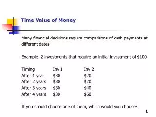
Alternative Solutions • A capital expenditure opportunity entails a cash outlay with the expectation of future benefits over time.

Alternative Solutions • To determine the worth of any alternative capital expenditure, four variables must be defined: • All relevant costs and the time when these expenditures will occur. • All benefits or revenues attributable to the expenditures and the time when they will occur. • The economic life of the alternative. • The prevailing interest rate at the time at which costs and revenues accrue.

Economic Life • The economic life of a capital expenditure is the number of years that this item will make a positive economic contribution.

Developing Cash Flow Profiles • The cash flow profile should include all cash items flowing into or out of a project. Each cash flow item must be identified specifically according to the time at which this flow occurs. The major items included are: • First cost, P, is the sum of the costs required to bring the asset into service • Salvage, V, is the net sum realized from the disposal of the asset at the termination of its economic life. • Income (revenues), other benefits and expenses.

Developing Cash Flow Profiles • Income, other benefits and expenses are identified according to their type of flow over time: • Periodic cash flow items occur at specific times (e.g., engine overhaul every three years) • Uniform series revenues or expenses are equal periodic amounts (e.g., property taxes, leasing costs, etc.) • Continuous revenues or expenses occurring uniformly over the life of the project (e.g., savings realized by replacing obsolete equipment)

Developing Cash Flow Profiles • Convention in engineering economy studies dictates that all discrete cash flows occur at the end of the period, normally at the end of the year. • To ensure that all positive and negative cash flow items are included in the analysis, and to better visualize these cash flows, it is useful to construct a cash flow diagram or table.

Developing Cash Flow Profiles A A A A A A A A 2 3 4 5 n-1 n 1 V P In Tabular Form...

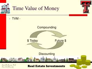
Interest Rate • When analyzing the feasibility of any investment, two principles must be observed. • First, the value of a sum of money is a function of the time span between the base point of reference and the date an expenditure or the receipt of revenue will occur (e.g., the value of $100 one year from today is not the same as $100 today). Consequently, money has a time value, which is measured by the interest rate. • Second, because of this time value of money, all comparisons must be made at a common point in time.

Interest Formulas • Interest formulas provide the mechanism for converting a cash flow at one specific time into an equivalent cash flow at another time. • Different formulas are used to compute problems involving discrete compound interest, continuously compounding interest, geometric series interest, and continuously compounding, continuous flow interest.

Simple Interest • The interest payment each year is found by multiplying the interest rate times the principal, I = Pi. After any n time periods, the accumulated value of money owed under simple interest, Fn, would be: • For example, $100 invested now at 9% simple interest for 8 years would yield • Nobody uses simple interest. Fn = P(1 + in) F8 = $100[1+0.09(8)] = $172

Compound Interest • The interest payment each year, or each period, is found by multiplying the interest rate by the accumulated value of money, both principal and interest.

Compound Interest • Consequently, the value for an amount P invested for n periods at i rate of interest using compound interest calculations would be: • For example, $100 invested now at 9% compound interest for 8 years would yield: • Compound interest is the basis for practically all monetary transactions. Fn = P( 1 + i )n F8 = $100( 1 + 0.09 )8 = $199

Nominal and Effective Interest Rates • Often it is appropriate to consider interest periods of one year. However, financial arrangements can call for interest to be compounded or paid more frequently, say quarterly, monthly or even daily. • Interest rates associated with compounding more frequently than annually are usually stated as “8% compounded quarterly,” for example.

Nominal and Effective Interest Rates • The nominal interest rate is expressed as an annual rate, without considering the effect of any compounding. It is obtained by multiplying the effective rate per interest period times the number of interest periods per year. • The effective annual interest rate is then the true or actual annual interest rate, taking into account the effect of compounding during the year.

Nominal and Effective Interest Rates • The nominal interest rate per year, r, is: where i is the effective interest rate per compounding period, and m is the number of compounding periods per year. • The effective interest rate per year, ia, is: r = im ia = ( 1 + i )m - 1, m < 

Nominal and Effective Interest Rates • For example, when the effective interest rate is 2% per month, the nominal interest rate per year is: • And the effective interest rate per year is: r = (0.02)(12) = 24% ia = (1 + 0.02)12 - 1 = 26.8%

Compound Interest FactorsDiscrete Cash Flow, Discrete Compounding • The notation used here is: • i = effective interest rate per interest period • n = number of compounding periods • A = end-of-period cash flows in a uniform series continuing for a specified number of periods. • F = future sum of money • P = present sum of money • The compound interest factors described in this section are used for discrete cash flows compounded discretely at the end of the period.

Compound Interest FactorsDiscrete Cash Flow, Discrete Compounding

Compound Amount Factor (Single Payment) • This factor finds the equivalent future worth, F, of a present investment, P, held for n periods at i rate of interest. • Example: What is the value in 9 years of $1,200 invested now at 10% interest

Compound Amount Factor (Single Payment) F 1 2 3 4 9 P = $1,200

Present Worth Factor (Single Payment) • This factor finds the equivalent present value, P, of a single future cash flow, F, occurring at n periods in the future when the interest rate is i per period (note: this factor is the reciprocal of the compound amount factor - single payment). • Example: What amount would you have to invest now to yield $2,829 in 9 years if the interest rate per year is 10%?

Present Worth Factor (Single Payment) F = $2,829 1 2 3 4 9 P

Compound Amount Factor(Uniform Series) • This factor finds the equivalent future value, F, of the accumulation of a uniform series of equal annual payments, A, occurring over n periods at i rate of interest per period. • Example: What would be the future worth of an annual year-end cash flow of $800 for 6 years at 12% interest per year?

Compound Amount Factor (Uniform Series) F 1 2 3 4 5 6 $800 $800 $800 $800 $800 $800

Sinking Fund Factor • This factor determines how much must be deposited each period in a uniform series, A, for n periods at i interest per period to yield a specified future sum. • Example: If a $1.2 million bond issue is to be retired at the end of 20 years, how much must be deposited annually into a sinking fund at 7% interest per year?

Sinking Fund Factor F = $1,200,000 1 2 3 4 20 A A A A A A

Capital Recovery Factor • This factor finds an annuity, or uniform series of payments, over n periods at i interest per period that is equivalent to a present value, P. • Example: What savings in annual manufacturing costs over an 8 year period would justify the purchase of a $120,000 machine if the firm’s minimum attractive rate of return (MARR) were 25%?

Capital Recovery Factor A A A A A 1 2 3 8 $120,000

Present Worth Factor(Uniform Series) • This factor finds the equivalent present value, P, of a series of end-of-period payments, A, for n periods at i interest per period. • Example: What lump sum payment would be required to provide $50,000 per year for 30 years at an annual interest rate of 9%?

Present Worth Factor(Uniform Series) $50,000 $50,000 $50,000 $50,000 $50,000 1 2 3 30 P

Arithmetic Gradient Conversion Factor(to Uniform Series) • Many times annual payments do not occur in equal amounts. If a series of payments increases by an equal amount, or gradient, each year, then a special compound interest factor can be used to reduce the gradient series to an equivalent equal-payment series. 3G 2G G 1 2 3 4

Arithmetic Gradient Conversion Factor(to Uniform Series) • The arithmetic gradient conversion factor (to uniform series) is used when it is necessary to convert a gradient series into a uniform series of equal payments. • Example: What would be the equal annual series, A, that would have the same net present value at 20% interest per year to a five year gradient series that started at $1000 and increased $150 every year thereafter?

Arithmetic Gradient Conversion Factor(to Uniform Series) 1 2 3 4 5 1 2 3 4 5 $1000 $1150 A A A A A $1300 $1450 $1600

Arithmetic Gradient Conversion Factor(to Present Value) • This factor converts a series of cash amounts increasing by a gradient value, G, each period to an equivalent present value at i interest per period. • Example: A machine will require $1000 in maintenance the first year of its 5 year operating life, and the cost will increase by $150 each year. What is the present worth of this series of maintenance costs if the firm’s minimum attractive rate of return is 20%?

Arithmetic Gradient Conversion Factor(to Present Value) $1600 $1450 $1300 $1150 $1000 1 2 3 4 5 P

Compound Interest FactorsDiscrete Cash Flow, Continuous Compounding • Monetary institutions and firms alike strive to keep their funds working at all times. • In the concept of discrete cash flows with continuous compounding, it is assumed that the cash flows occur once per year, but that compounding is continuous throughout the year.

Compound Interest FactorsDiscrete Cash Flow, Continuous Compounding • Thus if r = nominal interest rate per year M = number of compounding periods per year n = number of years • Then at the end of 1 year, one unit of principal will equal • Let k = M/r, then the above equation becomes

Compound Interest FactorsDiscrete Cash Flow, Continuous Compounding • The limit of (1+1/k)k as k approaches infinity is e. • Then the preceding equation can be rewritten as er, and the single payment continuous compounding amount factor at r percent nominal annual interest rate for N years is erN.

Compound Interest FactorsDiscrete Cash Flow, Continuous Compounding • Also, since erN (for continuous compounding) corresponds to (1+i)N for discrete compounding, er = 1 + i or i = er - 1 • By use of this relationship, the compound interest factors for discrete cash flows compounded continuously shown in the following table can be derived from the discrete compounding factors shown previously.

Compound Interest FactorsDiscrete Cash Flow, Continuous Compounding

Compound Interest FactorsContinuous Uniform Cash Flow, Continuous Compounding • Many cash flows can be assumed to occur continuously, such as accounts receivable, the cost of savings resulting from productivity improvements, or the costs of carrying inventories. Discrete 1 2 3 4 Continuous 1 2 3 4

Compound Interest FactorsContinuous Uniform Cash Flow, Continuous Compounding • Again, as with discrete cash flows, to solve for one variable given another, it is only necessary to select the proper interest factor for continuous cash flow, continuous compounding from the table on the next page. • In the following table, C represents the annual continuous cash flow (e.g., C = $20,000 represents a uniform series of continuous cash flows totaling $20,000 in one year).

Compound Interest FactorsContinuous Uniform Cash Flow, Continuous Compounding

Comparing Alternatives • One way to compare alternative investment strategies is in terms of the differences in cost or revenue relative to some reference time. • Two popular choices of time are Present and Future. • Present Worth • The present worth method compares all of a project’s estimated expenditures to all of its estimated revenues at a reference time called thepresent (t=0).

Present Worth • The present worth of alternative j with cash flows that last for n periods of time at i interest per period is: • If two or more alternatives are being compared, the alternative with the greatest present worth, or net present value, is recommended.

Present Worth • Example: Two pieces of equipment are being are being considered by a hospital to perform a particular service. • Brand A will cost $30,000 and will have an annual operating and maintenance cost of $5000 over its six year economic life, with a salvage value of $3000. • Brand B will cost $15,000, will have an annual operating and maintenance cost of $8000 over the first three years and $10,000 over the last three years of its economic life, and will have a negligible salvage value. • Which brand of equipment would you recommend, using the present worth comparison with an interest rate of 10% per year?

Present Worth In this example, Brand A would be the recommended alternative, since its present worth is greater.

Time Value of Money