Download
1 / 142
1.42k likes | 1.58k Vues
NEUTRINO OSCILLATIONS Luigi DiLella Physics Dept. and INFN, Pisa, Italy CHIPP PhD Winter School 2011. Formalism of neutrino oscillations in vacuum Solar neutrinos Neutrino oscillations in matter The KAMLAND reactor experiment “Atmospheric” neutrinos The Chooz reactor experiment

E N D
NEUTRINO OSCILLATIONS Luigi DiLella Physics Dept. and INFN, Pisa, Italy CHIPP PhD Winter School 2011 • Formalism of neutrino oscillations in vacuum • Solar neutrinos • Neutrino oscillations in matter • The KAMLAND reactor experiment • “Atmospheric” neutrinos • The Chooz reactor experiment • Long baseline oscillation searches at accelerators • Future projects: measurement of the q13 mixing angle • Puzzling results: LSND and MiniBooNE experiments
Neutrino oscillations in vacuum a = e, , (flavour index) i= 1, 2, 3 (mass index ) Uai : unitary mixing matrix Hypothesis: neutrino mixing (Pontecorvo 1958; Maki, Nakagawa, Sakata 1962) eare not mass eigenstates but linear superpositions of mass eigenstates 123with eigenvalues m1m2m3
Time evolution of a neutrino with momentum p produced in the flavour eigenstate naat time t = 0 Note: the complex phases are different if mjmk appearance of new flavour at time t > 0 Example for two – neutrino mixing mixing angle If at production (t = 0):
Probability to detect at time t if n(0) = : m2 m22 – m12 Using units more familiar to experimentalists: L = ct distance between neutrino source and detector Units:Dm2 [eV2]; L [km]; E [GeV] (or L [m]; E [MeV]) NOTE: Pab depends on Dm2 (not on m). If m1 << m2 , Dm2m22m12 m22 For m << p (in vacuum!)
Definition of oscillation length l: Units:l [km]; E [GeV]; Dm2 [eV2] (or l [m]; E [MeV]) E1, Dm21 E2, Dm22 sin2(2) Distance between neutrino source and detector E1 < E2 and/or Dm21> Dm22
Disappearance experiments Use na source, measure naflux at distance L from source Disappearance probability Examples: • Experiments using nefrom nuclear reactors (En few MeV: under threshold for m or t production) • nm detection at accelerators or in the cosmic radiation • (search for nm nt oscillations if En lower than t production threshold) The main source of systematic uncertainties: knowledge of the neutrino flux in the absence of oscillations use two detectors if possible n beam Far detector : measure Paa Near detector: measure n flux n source
Appearance experiments Neutrino source: na. Detect nb (b a) at distance L from source • Examples: • Detect ne + N e- + hadrons in a nm beam • Detect nt + N t - + hadrons in a nm beam (Threshold energy 3.5 GeV) • The nbcontamination at source must be precisely known (typically ne/nm 1% in nmbeams from high-energy accelerators) → a near detector is often very useful
Under the hypothesis of two – neutrino mixing: • Observation of an oscillation signal allowed parameter region in the[Dm2 , sin2(2)] plane consistent with the observed signal • No evidence for oscillation upper limit Pab< P exclusion region Very large Dm2 very short oscillation length l average over source and detector dimensions: log(Dm2) small Dm2 long l: L<<l (onset of the first oscillation) 0 1 sin2(2)
Searches for neutrino oscillations: experimental parameters
Solar neutrino deficit: ne disappearance between Sun and Earth • Convincing experimental evidence • Confirmation from a nuclear reactor experiment • Measurement of the oscillation parameters • “Atmospheric” neutrino deficit: nm , nmdisappearance in the cosmic • radiation over distances of the order of the Earth diameter • Convincing experimental evidence • Confirmation from long baseline accelerator experiments • Measurement of the oscillation parameters • LSND experiment at Los Alamos (1996): ne excess in a mixed • nm , nm, ne beam • To be confirmed – experimental results from the MiniBoone experiment • at Fermilab (designed to verify LSND) unclear and confusing EXPERIMENTAL EVIDENCE / HINTS FOR NEUTRINO OSCILLATIONS
Solar neutrinos Final result from a chain of fusion reactions in the Sun core: 4p He4 + 2e+ + 2ne Average energy produced as electromagnetic energy in the Sun core: Q = (4Mp– MHe4 + 2me)c2 – <E(2ne)> 26.1 MeV (<E(2ne)> 0.59 MeV) ( 2e+ + 2e– 4g ) Birth of a star: gravitational contraction of a primordial gas cloud (mainly 75% H2, 25% He) density, temperature increase in the star core NUCLEAR FUSION Hydrostatic equilibrium between pressure and gravity Solar luminosity: L = 3.846x1026 W = 2.401x1039 MeV/s Neutrino emission rate: dN(ne)/dt = 2L/Q 1.84x1038 s-1 Average neutrino flux on Earth: F(ne) 6.4x1010 cm-2 s-1 (average Sun - Earth distance = 1.496x10¹¹ m)
STANDARD SOLAR MODEL (SSM) (developed in 1960 and continuously updated by J.N. Bahcall and collaborators) Assumptions: • hydrostatic equilibrium • energy production by nuclear fusion • thermal equilibrium (power output = luminosity) • energy transport inside the Sun by radiation Input data: • cross-sections for fusion reactions • “opacity” (photon mean free path) as a function of distance • from the Sun center Method: • choice of initial parameters • evolution to present epoch (t = 4.6x10⁹ years) • compare predicted and measured quantities • modify initial parameters if necessary TODAY’S SUN: LuminosityL = 3.846x1026 W RadiusR = 6.96x10⁸ m Mass M = 1.989x1030 kg Core temperature Tc = 15.6x10⁶ K Surface temperature Ts = 5773 K Hydrogen in Sun core = 34.1%(initially 71%) Helium in Sun core = 63. 9%(initially 27.1%) as measured at the surface
Two reaction cycles p + p e+ + ne + d p + p e+ + ne + d OR (0.4%): p + e– + p ne + d p + d g + He3 p + d g + He3 He3 +He3 He4 + p + p OR (2x10⁻⁵): He3 + p He4 + e+ + ne p + p e+ + ne + d p + d g + He3 He3 +He4 g + Be7 p + Be7 g + B8 e– + Be7 ne + Li7 B8 Be8 + e+ + ne p + Li7 He4 +He4 Be8 He4 +He4 15% OR (0.13%) p – p cycle (0.985L) 85% CNO cycle (two branches) p + N15 C12 +He4 p + N15 g+O16 p + C12 g+N13 p + O16 g+F17 N13 C13 + e+ + ne F17 O17 + e+ + ne p + C13 g+N14 p + O17 N14 +He4 p + N14 g+O15 O15 N15 + e+ + ne NOTE #1: for both cycles 4p He4 + 2e+ + 2ne NOTE #2: source of today’s solar luminosity: fusion reactions occurring In the Sun core ~106 years ago (the Sun is a “main sequence star, practically stable over ~108 years).
Notations pp : p + p e+ + ne + d 7Be : e– + Be7 ne + Li7 pep : p + e– + p ne + d 8B : B8 Be8 + e+ + ne hep : He3 + p He4 + e+ + ne Mono-energetic lines: cm-2 s-1 Continuous spectra: cm-2 s-1 MeV -1 Predicted radial distribution of ne production in the Sun core Predicted solar neutrino flux and energy spectrum on Earth (p - p cycle)
The Homestake experiment (1970–1998): first detection of solar neutrinos A radiochemical experiment (R. Davis, University of Pennsylvania) ne + Cl 37 e– + Ar 37 Energy threshold E(ne) = 0.814 MeV Detector: 390 m3C2Cl4 (perchloroethylene) in a tank installed in the Homestake gold mine (South Dakota, U.S.A.) under 4100 m water equivalent (m w.e.) (fraction of Cl 37 in natural Chlorine = 24%) Expected production rate of Ar 37 atoms 1.5 per day Experimental method: every few months extract Ar 37 by N2 flow through tank, purify, mix with natural Argon, fill a small proportional counter, detect radioactive decay of Ar 37: e– + Ar 37 ne + Cl 37(half-life t1/2 = 34 d) (Final state excited Cl 37 atom emits Augier electrons and/or X-rays) Check efficiencies by injecting known quantities of Ar 37 into tank Results over more than 20 years of data taking SNU (Solar Neutrino Units): the unit to measure event rates in radiochemical experiments: 1 SNU = 1 event s–1 per 1036 target atoms Average of all measurements: R(Cl 37) = 2.56 0.16 0.16 SNU (stat) (syst) SSM prediction: 7.6 SNU Solar Neutrino Deficit +1.3 –1.1
“Real time” experiments with water Čerenkov counters Neutrino – electron elastic scattering:n + e– n + e– Detect Čerenkov light emitted by electrons in water Energy threshold ~5 MeV (5 MeV electron residual range in H2O 2 cm) Cross-sections: s(ne) 6 s(nm) 6 s(nt) nee- W e-ne • n • Z • e- (all threentypes) (ne only) W , Z exchange Z exchange only Two experiments: Kamiokande (1987 - 94) Fiducial volume: 680 m3 H2O Super-Kamiokande (1996 - ) Fiducial volume: 22500 m3 H2O in theKamioka mine (Japan) Depth2670 m H2O eq. The signal solar origin is demonstrated by the angular correlation between the directions of the detected electron and the incident neutrino cosqsun ~15 events / day In the peak
Super-Kamiokande detector Cylinder, height=41.4 m, diam.=39.3 m 50 000 tons of pure water Outer volume (veto) ~2.7 m thick Inner volume: ~ 32000 tons (fiducial mass 22500 tons) 11200 photomultipliers, diam.= 50 cm Light collection efficiency ~40% Inner volume while filling
Results from 22400 events (1496 days of data taking) Measured neutrino flux (assuming all ne): F(ne) = (2.35 0.02 0.08) x 106 cm-2 s –1 (stat) (syst) SSM prediction: F(ne) = (5.05 ) x 106 cm-2 s –1 Data/SSM = 0.465 0.005 (stat) +1.01 –0.81 +0.093 –0.074 ne DEFICIT (including theoretical error) Recoil electron kinetic energy distribution from ne– e elastic scattering of mono-energetic neutrinos is almost flat between 0 and 2En/(2 + me/En) convolute with predicted spectrum to obtain SSM prediction for electron energy distribution En SSM prediction Events/day Data 6 8 10 12 14 Electron kinetic energy (MeV)
Comparison of Homestake and Kamioka results with SSM predictions 0.465 0.016 2.56 0.23 Homestake and Kamioka results were known since the late 1980’s. However, the solar neutrino deficit was not taken seriously at that time. Why?
The two main solar ne sources in the Homestake and water experiments: He3 +He4 g + Be7 e– + Be7 ne + Li7 (Homestake) p + Be7 g + B8 B8 Be8 + e+ + ne (Homestake, Kamiokande, Super-K) Fusion reactions strongly suppressed by Coulomb repulsion Ec Z1Z2e2/d R1 d Potential energy: R2 Z1e Z2e d ~R1+R2 Ec 1.4 MeV for Z1Z2 = 4, R1+R2 = 4 fm Average thermal energy in the Sun core <E> = 1.5 kBTc 0.002 MeV (Tc=15.6 MK) kB (Boltzmann constant) = 8.6 x 10⁻⁵ eV/deg.K Nuclear fusion in the Sun core occurs by tunnel effect and depends strongly on Tc
Nuclear fusion cross-section at very low energies Nuclear physics term difficult to calculate measured at energies ~0.1– 0.5 MeV and assumed to be energy independent Tunnel effect: v = relative velocity Predicted dependence of the ne fluxes on Tc: From e– + Be7 ne + Li7: F(ne) Tc8 From B8 Be8 + e+ + ne : F(ne) Tc18 F TcN DF/F = N DTc/Tc How precisely do we know the temperature T of the Sun core? Search for ne from p + p e+ + ne + d (the main component of the solar neutrino spectrum, constrained by the Sun luminosity) very little theoretical uncertainties
Gallium experiments: radiochemical experiments to search for • ne + Ga71 e– + Ge71 • Energy threshold E(ne) > 0.233 MeV reaction sensitive to solar neutrinos • from p + p e+ + ne + d (the dominant component) • Three experiments: • GALLEX (Gallium Experiment, 1991 – 1997) • GNO (Gallium Neutrino Observatory, 1998 – ) • SAGE (Soviet-American Gallium Experiment) In the Gran Sasso National Lab 150 km east of Rome Depth 3740 m w.e. In the Baksan Lab (Russia) under the Caucasus. Depth 4640 m w.e. • Target: 30.3 tons of Gallium in HCl solution (GALLEX, GNO) • 50 tons of metallic Gallium (liquid at 40°C) (SAGE) • Experimental method: every few weeks extract Ge71 in the form of GeCl4 (a highly volatile • substance), convert chemically to gas GeH4, inject gas into a proportional counter, detect • radioactive decay of Ge71: e– + Ge71 ne + Ga71 (half-life t1/2 = 11.43 d) • (Final state excited Ga71 atom emits X-rays: detect K and L atomic transitions) • Check of detection efficiency: • Introduce a known quantity of As71 in the tank (decaying to Ge71: e– + Ge71 ne + Ga71) • Install an intense radioactive source producing mono-energetic ne near the tank: e– + Cr51 ne + V51 (prepared in a nuclear reactor, initial activity 1.5 MCurie equivalent to 5 times the solar neutrino flux),E(ne) = 0.750 MeV, half-life t1/2 = 28 d
Ge71 production rate ~1 atom/day +6.5 –6.1 SAGE (1990 – 2001) 70.8 SNU SSM PREDICTION: 128 SNU Data/SSM = 0.56 0.05 +9 –7
SNO Concluding evidence for solar neutrino oscillations (Sudbury Neutrino Observatory, Sudbury, Ontario, Canada) SNO: detector of Čerenkov light produced in 1000 tons of ultra-pure heavy water D2O contained in an acrylic sphere (diam. 12 m), surrounded by 7800 tons of ultra-pure water H2O Light collection: 9456 photomultipler tubes, diam. 20 cm, on a spherical surface of 9.5 m radius Depth: 2070 m (6010 m H2O eq.) in a Nickel mine Detection energy threshold: 5.5 MeV (reduced to 3.5 MeV in a recent analysis) Reconstruct the event position from the measurement of the photomultiplier signal relative timings
Solar neutrino detection in the SNO experiment (ES)Neutrino – electron elastic scattering : n + e– n + e– Directional,s(ne) 6 s(nm) 6 s(nt) (as in Super-K) (CC) ne + d e–+ p + p Electron angular distribution 1 - cos(qsun) Measurement of the ne energy (most of the ne energyis transferred to the electron) (NC) n + dn + p + n Identical cross-section for all three neutrino flavours ⇒ measurement of the total neutrino flux from B8 Be8 + e+ + n independent of oscillations 1 3 n H3 p DETECTION OFn + dn + p + n Detect neutron capture after “thermalization” • Phase I (November 1999– May 2001): n + d H3 +g( Eg= 6. 25 MeV, s = 5x10⁻⁴ b );g→ Compton electron, e+e- pair • Phase II (July 2001 – September 2003): add 2 tons of ultra-pure NaCl to D2O n + Cl35 Cl 36 +severalg’s ( <Ng> ≈ 2.5, S Eg 8. 6 MeV, s = 44 b ) • Phase III (November 2004 – November 2006: insert in the D2O volume an array of cylindrical proportional counters (diameter 5 cm) filled with He3 n + He3 p + H3 (0.764 MeV mono-energetic signal, s = 5330 b)
Neutron detection efficiency in Phase I and II Efficiency measurement using a Cf 252 neutron source (spontaneous fission, t½ = 2.6 years) Average over a spherical volume of radius R = 550 cm (50 cm from the edge of the D2O sphere) + 0.009 - 0.008 Detection efficiency for neutrons from n + d n + p + n = 0. 407 ± 0. 005 Efficiency without NaCl 0.14
. Phase II solar data An additional advantage of Phase II with respect to Phase I n + Cl35Cl36 +several g’s (on average, Ng = 2.5) The Čerenkov light is more isotropic with respect to the CC and ES reactions which have only one electron in the final state To measure the isotropy of the light emitted in each event define an an “isotropy parameter” b14 using the space distribution of photomultiplier hits 252Cf: neutron source (neutron energy: few MeV) 16N: g – ray source (6.13 MeV) Compton electron, collinear e+e- pair
Direct measurement of the electron angular resolution using the 16N g – ray source Compton electron T > 5. 5 MeV collinear with incident g Known source position g - ray 6.13 MeV
Use four independent variables to separate the three reactions ( Hatched histograms correspond to Phase II ) ES CC NC Teff Energy distribution (from signal amplitude) Cosqsun Directionality b14 Isotropy parameter r = (R/R0)3 Event radial position R0 = 600.5 cm radius of the D2O sphere
DATA cos qsun distribution Event position: distribution of distance from center r = (R / R0)3 R0 = 600.5 cm radius of D2O sphere
Energy distribution (from signal amplitude) Extract all components (ES, CC, NC, background) by maximum likelihood method Number of events: CC: 2176 ± 78 ES: 279 ± 26 NC: 2010 ± 85 Background from external neutrons: 128 ± 42
Solar neutrino fluxes, as measured from the three signals: FCC = ( 1.72 ± 0.05 ± 0.11 ) x10 6 cm -2 s -1 FES = (2. 34 ± 0.23 ) x10 6 cm -2 s -1 FNC = (4. 81 0. 19 ) x10 6 cm -2 s -1 Note: FCCF(ne) • 0.15 - 0.14 Calculated assuming that all incident neutrinos are ne +1.01 –0.81 • 0.28 - 0.27 FSSM( n) = 5.05 x 106cm-2s-1 (stat) (syst) differs from 1 by 10 standard deviations FCC FNC = 0.358 0.021 DEFINITIVE EVIDENCE OF SOLAR NEUTRINO OSCILLATIONS • 0.028 - 0.029 • The TOTAL solar neutrino flux agrees with SSM predictions (determination of the solar core temperature to ~ 0.5% precision) • Composition of solar neutrino flux on Earth: ~ 36% ne ; ~ 64% nm+nt (ratio nm/nt unkown)
SNO phase III B. Aharmim et al., Phys. Rev. Lett. 101, 111301 (2008) Insert 40 cylindrical proportional counters filled with He3 (NCD) vertically in the D2O volume (no salt) 36 Tubes filled with 85% He3, 15% CF4; 4 tubes filled with 85% He4, 15% CF4 Pressure 2.5 bar Ultra-pure Nickel tubes, diam. 5.08 cm Tube wall thickness 370 mm Variable length Detect neutrons from NC process n + d → n+ p + n from capture by He3 after thermalization • n + He3 → p + H3 + 764 KeV • mono-energetic signal • (~ 20,000 electron – ion pairs in gas) • detection efficiency ~18% • measured using Na24 sources (g, 2.754 MeV) • inserted in the D2O volume: • g + d → p + n • (neutron detection efficiency from n + d → H3 + g ≈ 4.9 %) Na24 calibration : Energy distribution Reduced signal amplitude for neutron captures near the tube wall
FCC FNC = 0.301 0.033 NCD energy distribution during Phase III data - taking (November 2004 – november 2006) Contamination from a radioactivity in the Nickel walls measured by the four counters filled with He4 Number of solar neutrino events: Neutrons: 983 ± 77 (NCD); 267 ± 23 (n + d → H3 + g) Electrons from CC events : 1867 ; electrons from ES events: 171 ± 24 Background neutrons: 185 ± 24 (NCD); 77 ± 12 (n + d → H3 + g) +91 -101 Measurement of the solar ne deficit using an independent method with different systematic effects
Solar ne disappearance: interpretation Check dependence of Pee on E and L Hypothesis: two – neutrino mixing Vacuum oscillations ne energy spectrum measured on Earth F(ne) = Pee F0(ne) (F0(ne)ne energy spectrum at production) Probability to detect ne on Earth: L [m] E [MeV] Dm2 [eV2] Solar neutrino energy in SNO, Super-K experiments E = 5 – 15 MeV Variation of Sun – Earth distance during data taking (the Earth orbit is an ellipse) DL = 5.01 x 10⁹ m ( <L> = 149.67x 10⁹ m)
Spectral distortions Super-K 2002 Data/SSM Electron kinetic energy (MeV) SNO: ne + d e–+ p + p electron energy distribution SNO: data / SSM prediction nedeficit independent of energy within measurement errors (no spectral distortions)
Seasonal modulation Yearly variation of the Sun - Earth distance: 3.3% seasonal modulation of the solar neutrino flux 2 Expected seasonal variation from the variation of solid angle in the absence of oscillations: ~ 6.6% Days from start of data taking The observed effect is consistent with the expected solid angle variation
Neutrino oscillations in vacuum do not describe the observed solar ne deficit For oscillation lengths l << n source dimension (~ 0.15 RO ≈ 1 x 10⁸ m); << Earth diameter (~ 1.3 x 10⁷ m) Pee is independent of E and L : L [m] E [MeV] Dm2 [eV2] in disagreement with the experimental result ~ 0.33
NEUTRINO OSCILLATIONS IN MATTER p: neutrino momentum N: density of scattering centers f(0): scattering amplitude at = 0° In vacuum: Energy conservation: V neutrino potential energy in matter Neutrino refractive index in matter (L. Wolfenstein, 1978) Plane wave in matter: = ei(np•r–E’t) (|e | <<1) V<0: attractive potential (n>1) V>0: repulsive potential (n<1)
Neutrino potential energy in matter 1. Z-boson exchange (the same for the three neutrino types) n n Z GF: Fermi constant Np (Nn): proton (neutron) density w: weak mixing angle e,p,n e,p,n 2. W- boson exchange (only for ne!) ne e- W+ matter density [g/cm3] electron density e- ne NOTE: V(n) = – V( n )
Evolution equation: In the “flavour” representation: 2x2 matrix (Remember: for M p) NOTE: m1, m2, are defined in vacuum Example: ne–nm mixing in a constant density medium (identical results for ne–nt mixing)
Term inducing ne–nm mixing r = constant H is time - independent H diagonalization eigenvalues and eigenvectors diagonal term: no mixing Eigenvectors in matter [eV2] (r in g/cm3, E in MeV) Mixing angle in matter: x = Dm2cos 2qxres maximum mixing (qm = 45°) even if the mixing angle in vacuum is very small: “MSW resonance ” (discovered by Mikheyev and Smirnov in 1985)
Mass eigenvalues as a function of x M2 m22 m12 Oscillation length in matter: (l oscillation length in vacuum) For x = xres: NOTE: for ne oscillations the MSW resonanceexists only if Dm2cos2q > 0 Dm2 > 0, cos2q > 0 (q < 45º) or Dm2 < 0, cos2q < 0 (q > 45º) DEFINITION (to remove the ambiguity): Dm2 = m22 – m12 > 0
100 10 1 0.1 Solar density r [g/cm3] Oscillations in solar matter Time evolution:Hn= i n / t H (2 x 2 matrix) depends on time via r(t) H has no eigenvectors R/RO Numerical solution of the evolution equation: 0. 0.2 0.4 0.6 0.8 (pure ne at production) (d = very small time interval) (until the neutrino emerges from the Sun) Matter effects in solar neutrino oscillations Solar neutrinos are produced in a high – density medium (the solar core). Variable density along the neutrino path: r = r(t)
“Adiabatic solutions” (Negligible variation of matter density r over an oscillation length) Dm2 [eV2] r [g/cm3] x > xres n1(t) , n1(t) : “local” mass eigenstates obtained by setting r = constant = local density at time t in the evolution Hamiltonian constant along the whole path inside the Sun mixing angle in matter at neutrino production point (in the Sun core) Assumption: mixing angle in vacuum q <45° →cosq >sinq ; cos2q > 0 Mixing angle in matter: at production
M2 qm < 45° qm > 45° In case of “adiabatic” solutions, at exit from Sun ( t = tE ): n1( tE ), n2( tE ) : mass eigenstates in vacuum In vacuum, at exit from Sun (t = tE): ne DEFICIT
Day – night modulation (from matter effects on neutrino oscillations through Earth at night ne flux increase at night for some values of the oscillation parameters ) cos(Sun zenith angle) SNO: Day and Night spectra (CC events) Day – night difference Study ne deficit as a function of path inside Earth (length and density) subdividing the night spectrum in bins of zenith angle (with respect to local vertical axis)
“Best fit” to SNO data Confidence levels for two-parameter fits CL Dc2=c2-c2min • 68.27% 2.30 • 90% 4.61 • 95% 5.99 • 99% 9.21 • 99.73% 11.83 Best fit: NOTE: tan2q is used instead of sin22qbecause sin22qis symmetric around q = 45° MSW solutions exist only if q< 45°