WinRiver
WinRiver. 1. Average data to a greater interval Use raw data Decreases errors and increases data quality. 2. Convert to ASCII format Files found at: http://users.coastal.ufl.edu/~arnoldo/eoc6934/ponce/adcp /. depth cell length (cm). Bottom track vel (east in cm/s).

WinRiver
E N D
Presentation Transcript
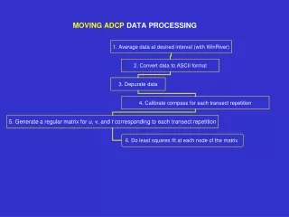
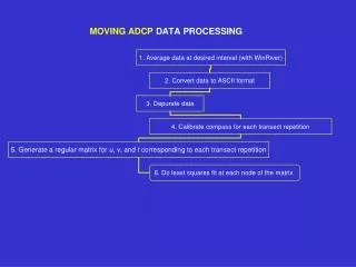
1. Average data to a greater interval Use raw data Decreases errors and increases data quality
2. Convert to ASCII format Files found at: http://users.coastal.ufl.edu/~arnoldo/eoc6934/ponce/adcp/
depth cell length (cm) Bottom track vel (east in cm/s) time per ensemble (hundredths of s) Profiling mode # of depth cells Ensemble # # of ensembles in segment pitch roll ADCP depth blank after transmit (cm) corrected heading temperature Total elapsed time (s) # of pings per ensemble Bottom track vel (vertical in cm/s) Bottom track vel (error in cm/s) Total elapsed distance (m) Distance traveled north (m) Distance traveled east (m) Course made good (m) Bottom track vel (north in cm/s) Ship velocity north (cm/s) Ship velocity east (cm/s) Total distance traveled (m) # of bins to follow and units of measurement Velocity reference (BT, layer, none) and intensity units (dB or COUNTS) Intensity scale factor (dB/count) Sound absorption factor (in dB/m) Date and time Discharge Values Depth Reading (m) Water layer vel Lat & Lon % good Velocity Magnitude Velocity Direction East Component North Component Vertical Error Echo Intensity Discharge Bin depth
3. Depurate data with the following criteria (for Lily Springs): % good > 20% |error| < 10 cm/s
3. Depurate data with the following criteria (for other data): % good > 80% |error| < 10 cm/s discharge < 100 m3/s ship speed or bottom track speed > 0.15 m/s
4. Calibrate Compass Method of Joyce (1989, Journal of Atmospheric and Oceanic Technology, 6, 169-172) and Method of Pollard & Reid (1989) tan =< ubtvsh - vbtush>/<ubtush + vbtvsh> 1 + = [<ush2 + vsh2>/<ubt2+ vbt2>]1/2 ucorr = [1 + ][u cos - v sin ] vcorr = [1 + ][u sin + v cos ] where ubt is the East component of the bottom track velocity ush is the East component of the navigation velocity (from GPS) u is the East component of the current velocity measured by the ADCP ucorr is the corrected East component of velocity < > indicates average throughout one transect repetition Carry out the correction for each transect repetition
5. Generate a regular matrix for u, v, and t corresponding to each transect repetition Identify each transect repetition according to the time of beginning and end of each repetition
Draw each repetition placing the data (u, v, andt) on a regular grid (distance vs. depth) The origin of the matrix (zero distance) is arbitrary (e.g. a point at the coast) Calculate the distance from that origin to the location of each profile in order to generate the regular grid The end result is a group of Nregular grids, whereNis the number of transect repetitions. Each grid point has a time series ofNvalues foru,v, t, andbackscatter.