Decision Tree Algorithms in Classification
Understand the power of decision trees for classification and prediction, and learn about entropy, information gain, and attribute selection methods. Example scenarios and a decision tree illustration included.

Decision Tree Algorithms in Classification
E N D
Presentation Transcript
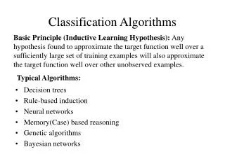
Classification Algorithms Decision Tree Algorithms
The problem • Given a set of training cases/objects and their attribute values, try to determine the target attribute value of new cases. • Classification • Prediction
Why decision tree? • Decision trees are powerful and popular tools for classification and prediction. • Decision trees represent rules, which can be understood by humans and used in knowledge system such as database.
key requirements • Attribute-value description:object or case must be expressible in terms of a fixed collection of properties or attributes (e.g., hot, mild, cold). • Predefined classes (target values):the target function has discrete output values (Boolean or multiclass) • Sufficient data:enough training cases should be provided to learn the model.
Random split • The tree can grow huge • These trees are hard to understand. • Larger trees are typically less accurate than smaller trees.
Principled Criterion • Selection of an attribute to test at each node - choosing the most useful attribute for classifying examples. • information gain • measures how well a given attribute separates the training examples according to their target classes • This measure is used to select among the candidate attributes at each step while growing the tree
Entropy • A measure of homogeneity of the set of examples. • Given a set S of positive and negative examples of some target concept (a 2-class problem), the entropy of set S relative to this binary classification is E(S) = - p1*log2 p1 – p2*log2 p2
Example • Suppose S has 25 examples, 15 positive and 10 negatives [15+, 10-]. Then the entropy of S relative to this classification is E(S)=-(15/25) log2(15/25) - (10/25) log2 (10/25)
Entropy • Entropy is minimized when all values of the target attribute are the same. • If we know that Joe always plays Center Offence, then entropy of Offence is 0 • Entropy is maximized when there is an equal chance of all values for the target attribute (i.e. the result is random) • If offence = center in 9 instances and forward in 9 instances, entropy is maximized
Information Gain • Information gain measures the expected reduction in entropy, or uncertainty. • Values(A) is the set of all possible values for attribute A, and Sv the subset of S for which attribute A has value v Sv = {s in S | A(s) = v}. • the first term in the equation for Gain is just the entropy of the original collection S • the second term is the expected value of the entropy after S is partitioned using attribute A
Information Gain • It is simply the expected reduction in entropy caused by partitioning the examples according to this attribute. • It is the number of bits saved when encoding the target value of an arbitrary member of S, by knowing the value of attribute A.
Examples • Before partitioning, the entropy is • H(10/20, 10/20) = - 10/20 log(10/20) - 10/20 log(10/20) = 1 • Using the ``where’’ attribute, divide into 2 subsets • Entropy of the first set H(home) = - 6/12 log(6/12) - 6/12 log(6/12) = 1 • Entropy of the second set H(away) = - 4/8 log(4/8) - 4/8 log(4/8) = 1 • Expected entropy after partitioning • 12/20 * H(home) + 8/20 * H(away) = 1
Using the ``when’’ attribute, divide into 3 subsets • Entropy of the first set H(5pm) = - 1/4 log(1/4) - 3/4 log(3/4); • Entropy of the second set H(7pm) = - 9/12 log(9/12) - 3/12 log(3/12); • Entropy of the second set H(9pm) = - 0/4 log(0/4) - 4/4 log(4/4) = 0 • Expected entropy after partitioning • 4/20 * H(1/4, 3/4) + 12/20 * H(9/12, 3/12) + 4/20 * H(0/4, 4/4) = 0.65 • Information gain 1-0.65 = 0.35
Decision • Knowing the ``when’’ attribute values provides larger information gain than ``where’’. • Therefore the ``when’’ attribute should be chosen for testing prior to the ``where’’ attribute. • Similarly, we can compute the information gain for other attributes. • At each node, choose the attribute with the largest information gain.
Outlook Sunny Overcast Rain Humidity Wind Yes Strong High Normal Weak No Yes No Yes Decision Tree: Example Day Outlook Temperature Humidity Wind Play Tennis 1 Sunny Hot High Weak No 2 Sunny Hot High Strong No 3 Overcast Hot High Weak Yes 4 Rain Mild High Weak Yes 5 Rain Cool Normal Weak Yes 6 Rain Cool Normal Strong No 7 Overcast Cool Normal Strong Yes 8 Sunny Mild High Weak No 9 Sunny Cool Normal Weak Yes 10 Rain Mild Normal Weak Yes 11 Sunny Mild Normal Strong Yes 12 Overcast Mild High Strong Yes 13 Overcast Hot Normal Weak Yes 14 Rain Mild High Strong No
Weather Data: Play or not Play? Note: Outlook is the Forecast, no relation to Microsoft email program
Example Tree for “Play?” Outlook sunny rain overcast Yes Humidity Windy high normal false true No Yes No Yes
Example: attribute “Outlook” • “Outlook” = “Sunny”: • “Outlook” = “Overcast”: • “Outlook” = “Rainy”: • Expected information for attribute: Note: log(0) is not defined, but we evaluate 0*log(0) as zero
Computing the information gain • Information gain: (information before split) – (information after split) • Information gain for attributes from weather data:
The final decision tree • Note: not all leaves need to be pure; sometimes identical instances have different classes Splitting stops when data can’t be split any further
Determining the Best Attribute Entropy(S) = -pcinema log2(pcinema) -ptennis log2(ptennis) – pshopping log2(pshopping) –pstay_in log2(pstay_in) = -(6/10) * log2(6/10) -(2/10) * log2(2/10) -(1/10) * log2(1/10) -(1/10) * log2(1/10) = -(6/10) * -0.737 -(2/10) * -2.322 -(1/10) * -3.322 -(1/10) * -3.322 = 0.4422 + 0.4644 + 0.3322 + 0.3322 = 1.571 and we need to determine the best of: Gain(S, weather) = 1.571 - (|Ssun|/10)*Entropy(Ssun) – (|Swind|/10)*Entropy(Swind) – (|Srain|/10)*Entropy(Srain) = 1.571 - (0.3)*Entropy(Ssun) - (0.4)*Entropy(Swind) – (0.3)*Entropy(Srain) = 1.571 - (0.3)*(0.918) - (0.4)*(0.81125) - (0.3)*(0.918) = 0.70 Gain(S, parents) = 1.571 - (|Syes|/10)*Entropy(Syes) - (|Sno|/10)*Entropy(Sno) = 1.571 - (0.5) * 0 - (0.5) * 1.922 = 1.571 - 0.961 = 0.61 Gain(S, money) = 1.571 - (|Srich|/10)*Entropy(Srich) - (|Spoor|/10)*Entropy(Spoor) = 1.571 - (0.7) * (1.842) - (0.3) * 0 = 1.571 - 1.2894 = 0.2816
Now we look at the first branch. Ssunny = {W1, W2, W10}, not empty and the class labels for these rows are not common, thus we put a node rather than a leaf. Samething is for the 2nd and 3rd branches (Weather, windy) and (weather, rainy), and therefore, we put a node for each one of them.
Now we focus on the first branch of the tree data, i.e. data for attribute values (Weather, Sunny) as shown below: Hence we can calculate: Gain(Ssunny, parents) = 0.918 - (|Syes|/|S|)*Entropy(Syes) - (|Sno|/|S|)*Entropy(Sno) = 0.918 - (1/3)*0 - (2/3)*0 = 0.918 Gain(Ssunny, money) = 0.918 - (|Srich|/|S|)*Entropy(Srich) - (|Spoor|/|S|)*Entropy(Spoor) = 0.918 - (3/3)*0.918 - (0/3)*0 = 0.918 - 0.918 = 0
Remembering that we replaced the set S by the set S(Sunny), looking at S(yes), we see that the only example of this is W1. Hence, the branch for yes stops at a categorisation leaf, with the category being Cinema. Also, S(no) contains W2 and W10, but these are in the same category (Tennis). Hence the branch for no ends here at a categorisation leaf. Hence our upgraded tree looks like this: Finishing this tree off is left as a tutorial exercise.