Activator - Ch. 4 Sec 1

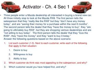
1. Activator - Ch. 4 Sec 1 • Three people enter a Mazda dealership all interested in buying a brand new car. All three initially stop to look at the Mazda RX8. The first person tells the salesperson that they “really like the RX8” but they “don’t have any money today”, and are “saving their money for a purchase within the next 6 months”. The second person tells the dealer that they “have the money to buy”, they “are going to ultimately buy RX8”, but they are shopping various dealerships and are “not willing to buy today”. The third person tells the dealer that they “love the RX8!”, they “have the money” and they “want to buy it today.”Answer the following questions based on the above scenario: • List each customer (1-3). Next to each customer, write each of the following that apply to their situation: • Desire to buy • Willingness to buy • Ability to buy • Which customer do think was most appealing to the salesperson, and why? • Which customer would you have helped first, and why?

2. Chapter 4 - DemandSection 1 – Understanding Demand • Demand – desire, ability, and willingness to buy a good/service • The amount of a product that a consumer (individual) or group of consumers (market) will purchase at a given price • In a market system, buyers and sellers determines the prices of goods and services • Microeconomics – The study of the economic behavior and decision making of small units, such as individuals, families, and firms (businesses)

3. Application Chart – Demand • Make a three column chart that represents 3 items that you want on one side, whether you can afford them or not in the next, and whether you are willing to buy them in the last.

4. The Law of Demand Price Prices of ProductsDecreases DemandQuantity Demanded Increases • Law of Demand –prices are lower, consumers will buy more; prices are higher, consumers will buy less. • Inverse relationship between price and the QD of a product. • Prices strongly influence the quantity demanded of a product PricePrices of Product Increases Demand Quantity DemandedDecreases

5. Change in Quantity Demanded $3.50 $1.00

6. Change in Quantity Demanded $1.00 $3.50

7. The Income Effect • Income Effect – the change in consumption resulting from a change in price, “more bang for your buck” • Consumers feel richer when prices drop, poorer when prices rise. Both affect the Quantity Demanded of a product.

8. The Income Effect Purchases http://www.youtube.com/watch?v=JC7KB-HF6ao&feature=related http://www.youtube.com/watch?v=_87YZPSdHX8&feature=related More Bang for your Buck http://www.youtube.com/watch?v=4hZ9g4xo24A&feature=player_detailpage#t=2s

9. Substitution Effect • Substitution Effect – when consumers react to an increase in a good’s price by consuming less of one good and more of other goods $3.99 $4.99 $3.99

10. The Demand Schedule • Demand Schedule - a table that lists the quantity of a good that a person will purchase at each price in a market • Market Demand Schedule - lists the quantity of a good that all consumerswill purchase at each price in the market

11. Price per Ice Cream Cone $3.00 2.50 2.00 1.50 1.00 0.50 0 1 2 3 4 5 6 7 8 9 10 11 12 Quantity Demanded of Ice-Cream Cones per week Application - The Demand Curve • Demand Curve - graphically represents the demand schedule • Demand Curve is downward sloping because of the law of demand

12. Price per Ticket $40.00 30.00 25.00 20.00 15.00 10.00 0 2 4 6 8 10 12 14 16 18 20 22 24 Quantity Demanded of Tickets Chapter 4 Section 2 Plot the demand schedule below, which represents 2004 Florida Marlins avg. sales per game (in thousands) 35.00 D3 D1 D2

13. Section 2 - Shifts of the Demand Curve Price • Changes in Demand are reflected as a shift in the curve • Shifts to the right indicate an increase in demand • Shifts to the left indicate a decrease in demand Increase in demand Decrease in demand Demand curve, D 2 Demand curve, D 1 Demand curve, D 3 0 Quantity Demanded

14. Difference Between A Change in Quantity Demanded and a Change in Demand • QD - A change in the amount a consumer will purchase as a result of a change in price (ceteris paribus – all other things constant) • Reflected as movement along the curve • D – A change in the amount a person will buy as a result of an outside factor (change in ceteris paribus - popularity of product, consumer income, etc.) • Reflected as a shift in the curve

15. Flow Chart – Determinants of Demand – pgs. 85 - 87 What Causes a Shift? Consumer Income Consumer Expectations Population Consumer Tastes and Advertising Price of Related Goods DescriptionConsumer Income has a major influence on a consumer’s demand Description Description Description Description Example of Increase DemandPeople are paid more, they buy more normal goods Example of Increase Demand Example of Increase Demand Example of Increase Demand Example of Increase Demand Example of Decrease Demand People are paid less they buy less normal goods and more inferior goods Example of Decrease Demand Example of Decrease Demand Example of Decrease Demand Example of Decrease Demand

16. What Causes a Shift? • Consumer Income • Consumer Expectations • Population • Consumer Tastes and Advertising • Price of Related Products Group Assignment (pg. 86-88): Create a scenario that represents each of the five determinants of demand. Provide a scenario that shifts the demand curve to the right and the left.

17. Consumer Income • Consumer Income – A consumer’s income affects their demand for most goods and services • Increase in income will cause an increase in consumption • Decrease in income will cause a decrease in consumption • Normal good – • Inferior good –

18. Price of Related Goods • Price of related goods – demand for goods can be affected by the price for related goods • Complements – the demand of one good increases as a result of the purchase of another good • Substitutes – the demand for one good decreases because another good is used in its place

19. Consumer Tastes and Advertising • Consumer Tastes and Advertising – changes in popularity of products or the influence of trends and advertising can affect demand • Popularity of product decreases, decreases in demand • Popularity of a product increases, increases in demand http://www.youtube.com/watch?v=4OhrQMnOYOQ&feature=player_detailpage#t=34s http://www.youtube.com/watch?v=m02-lyUOH5M&feature=player_detailpage#t=61s

20. Consumer Expectations • Consumer Expectations – refers to the way people think about the future, as it relates to consumption • Expectations for the future can affect consumption for the present

21. Population • Population – an increase in the number of consumers can cause an increase or decrease in the demand for products • Increase in population, increase in demand • Decrease in population, decrease in demand

22. Price per SUV $55 30 25 20 15 10 0 2 4 6 8 10 12 14 16 18 20 Quantity Demanded of SUVs Demand Application – Average sales of SUV’s per month (in millions) • Plot the demand schedule below. The graph represents the demand for SUV’s during the early 1990’s. During the late 1990’s SUV’s became increasingly popular in the United States. During the mid 2000’s, gas prices increased nationally to average rates around 5.00 per gallon. Consumers expected these prices to remain in the future, which affected the demand for SUV’s around the country. 50 45 40 35

23. Price per SUV $55 30 25 20 15 10 0 2 4 6 8 10 12 14 16 18 20 Quantity Demanded of SUVs Demand Application – Average sales of SUV’s per month (in millions) How did the curve change from the early 90’s to the late 90’s What was the cause of the change from the early 90’s to the late 90’s? What happened to the curve after the gas hikes? 50 45 40 35 D3 D2 D1

24. Chapter 4 Section 3 • List 2 items that you would buy less of if the price increased • List 2 items that you would buy more of if the price decreased • List 2 items that you would continue to buy, even if the increased

25. Section 3 – Elasticity of Demand • Elasticity of Demand –how consumers will cut back or increase their quantity demanded for a product when prices rise or fall • Measures the extent to which changes in price causes changes in quantity demanded. • Helps determine how much a price change will influence the qd of any given product

26. Elastic Demand • Elastic – consumption changes drastically when a price rises or falls • A consumer is very responsive to price changes

27. Inelastic Demand • Inelastic - changes in price causes a relatively small change in quantity demanded • Consumers continue to purchase regardless of price change

28. Determinants of Demand Elasticity • Availability of Close Substitutes • Pepsi/Coke, Butter/Margarine • Relative Importance • How much you spend on a good • Table salt versus designer clothes • Necessities versus Luxuries • Medicine versus a luxury automobile • Change over time • Longer time horizon – more elastic • Gas in the short run is inelastic, but over time elastic

29. Values of Elasticity • Elasticity has a precise mathematical definition • Percentage change in quantity demanded Percentage change in price • Value is less than 1, it is considered inelastic. • Inelastic – Demand is < 1 • Value is greater than one, demand is elastic. • Elastic – Demand is > than 1 • Value is equal to one, demand is unitary elastic. • Unitary Elastic – Demand is = 1

30. Price $10.00 8.00 8 10 0 Quantity The Midpoint Method (Q2 – Q1) / [(Q2+Q1) / 2] (P2 – P1) / [(P2 + P1) / 2] Price Elasticity = A = .22 $10 – 8_ $9 10 – 8_ 9 = .22 B A B 22% 22% = 1 Unitary Elastic $10 – 8 9 = .22 10 – 8__ 9 = .22 A B .22 .22 Unitary Elastic = 1

31. Price $7.00 6.00 5.00 3.00 2.00 1.00 0 5 10 15 20 25 30 35 Quantity Demanded of Ice-Cream Cones per week Application – Elasticity of Ice Cream Cones (Q2 – Q1) / [(Q2+Q1) / 2] (P2 – P1) / [(P2 + P1) / 2] Price Elasticity = (Q2 – Q1) / [(Q2+Q1) / 2] 20 – 10 15 = .67 $4 – 3 $3.5 = .29 (P2 – P1) / [(P2 + P1) / 2] .67_ .29 = 2.3 • % change in qd % change in price 4.00 Elastic

32. Price $7.00 6.00 5.00 3.00 2.00 1.00 0 5 10 15 20 25 30 35 Quantity Demanded of Table Salt Application – Elasticity of Table Salt (Q2 – Q1) / [(Q2+Q1) / 2] (P2 – P1) / [(P2 + P1) / 2] Price Elasticity = 15 – 10 12.5 = .40 (Q2 – Q1) / [(Q2+Q1) / 2] $6 – 2 $4 = 1 (P2 – P1) / [(P2 + P1) / 2] 40 100 = .4 • % change in qd % change in price 4.00 Inelastic

33. Total Revenue • Total Revenue – the amount paid by buyers and received by sellers of a good • Price of the goods x quantity demanded = Total Revenue

34. Elasticity Application 1 (Q2 – Q1) / [(Q2+Q1) / 2] (P2 – P1) / [(P2 + P1) / 2] • Use the formula to show how you determine elasticity of demand for the graph. • Q2 _______ - Q1_______ = ______ / Q2 ______+ Q1 _______ / 2 = _______ = ________ • P2 _______ - P1_______ = ______ / P2 ______+ P1 _______ / 2 = _______ = ________ • - Elasticity QD______ P______P = ________ • Did the price change cause an elastic or inelastic response in the QD for ice cream cones? ________________________________________________ 20 10 10 20 10 15 .67 5 3 2 5 3 4 .50 .67 . 50 1.34 Elastic

35. Elasticity Application 2 (Q2 – Q1) / [(Q2+Q1) / 2] (P2 – P1) / [(P2 + P1) / 2] • Use the formula to show how you determine elasticity of demand for the graph. • Q2 _______ - Q1_______ = ______ / Q2 ______+ Q1 _______ / 2 = _______ = ________ • P2 _______ - P1_______ = ______ / P2 ______+ P1 _______ / 2 = _______ = ________ • - Elasticity QD______ P______P = ________ • Did the price change cause an elastic or inelastic response in the QD for insulin? ________________________________________________ 8 5 3 8 5 6.5 .46 6 2 4 6 2 4 1 .46 1 .46 Inelastic

36. Scenario: The Apple store in St. John’s Mall made the decision to drop the price of their Ipod Nano from $150 to $125. As a result, the sale of Nano’s increased from 200 a week to 250. - Create a Demand Schedule and Curve based on the above information. Elasticity Application 3 Price Per Ipod Nano 150 125 150 125 200 250 200 250 • Use the formula to show how you determine elasticity of demand for the graph. • Q2 _______ - Q1_______ = ______ / Q2 ______+ Q1 _______ / 2 = _______ = ________ • P2 _______ - P1_______ = ______ / P2 ______+ P1 _______ / 2 = _______ = ________ • - Elasticity QD______ P______P = ________ 250 200 50 250 200 225 .22 150 125 25 150 125 137.5 .18 .22 .18 1.22 QD 0 Elastic 2. Did the price change cause an elastic or inelastic response in the QD for Nano’s? ___________________ 3. If the firm drops their price by _________%, they will see an increase in sales of __________% 4. To determine if this is a good decision for the firm, calculate the total revenue of each price: - Multiply the first price of the Nano by the first QD – $______ x _______ = ___________________ - Multiply the second price of the Nano by the second QD – $ ______ x _______ = __________________ 5. Which price point generates the most total revenue? ______________________ 18 22 150 200 $30,000 125 250 $31250 125

37. .18 • What is the price elasticity of demand when the price changes from $1 to $2? _________*Use the midpoint method formula to determine the answer to #1* • Q2 – Q1__ ________ (Q2 + Q1)/2 = ________________ = ___________ P2 – P1__ ________ (P2 + P1)/2 20 .12 170 1 .67 1.5 Based on the above result, demand for Moonbucks coffee at this price range is (elastic/unit elastic/inelastic)

38. 1.22 • What is the price elasticity of demand when the price changes from $5 to $6? _________*Use the midpoint method formula to determine the answer to #1* • Q2 – Q1__ ________ (Q2 + Q1)/2 = ________________ = ___________ P2 – P1__ ________ (P2 + P1)/2 20 .22 90 1 .18 5.5 Based on the above result, demand for Moonbucks coffee at this price range is (elastic/unit elastic/inelastic)

39. Price $10.00 8.00 8 10 0 Quantity The Midpoint Method (Q2 – Q1) / [(Q2+Q1) / 2] (P2 – P1) / [(P2 + P1) / 2] Price Elasticity = A = .22 $10 – 8_ $9 10 – 8_ 9 = .22 B A B 22% 22% = 1 Unitary Elastic $10 – 8 9 = .22 10 – 8__ 9 = .22 A B .22 .22 Unitary Elastic = 1

40. Price $10.00 8.00 8 10 0 Quantity The Flaw in Point Elasticity of Demand Elasticity = Percentage change in Quantity Demanded/Percentage change in Price % Q% P A = 25% $8 – 10 X100 $8 10 – 8 X 100 10 = 20% B A B 20% 25% = .8 Inelastic $10 – 8 X100 $10 = 20% 8 – 10 X 100 8 = 25% A B 25% 20% = 1.25 Elastic

41. Determinants of Demand Elasticity • Can The Purchase Be Delayed? • Insulin, gas, cigarettes, etc… • 2. Are Adequate Substitutes Available? • Pepsi/Coke, Steaks/Chicken, etc… • 3. Does the Purchase Use a Large Portion of Income? • Table Salt vs. Automobiles

42. Law of Diminishing Marginal Utility • Diminishing Marginal Utility – a decrease in the (utility) usefulness due to the reduced satisfaction of a product. • Utility – usefulness of a good/service to a consumer.

43. Law of Diminishing Marginal Utility get 2nd ½ price Buy 1 pair

44. Do Now – Ch. 5 Sec 1 • Following graduation, Braden McElroy opens a smoothie shop called, . Initially, he needs to determine the products that he wishes to sell at the shop. He decides that he will offer 5 main types of smoothies on his menu • Braden’s Berry Blastoff • Braden’s Banana Bonanza • St. Simon’s Succulent Strawberries • Brunswick’s Blueberry Lagoon • Mocha Marsh Surprise • During the first month of operation he offered all of his smoothies at 3.99. He found that people were willing to purchase “Braden’s Berry Blastoff”, “Braden’s Bananza Bonanza” and “St. Simon’s Succelent Strawberries”. Ultimately, Mocha Marsh Surprise sold very little, and he could barely keep “Brunswick’s Blueberry Lagoon in stock. • What should Braden do with the price of #’s 1, 2, and 3? • What should he do with the price of #4? • What might he do with number 5?

45. Application – Revenue Table • Revune – amount of money a company receives by selling its goods • Price of the goods x quantity demanded = Total Revenue

46. Application – Revenue Table • Revune – amount of money a company receives by selling its goods • Price of the goods x quantity demanded = Total Revenue