Robust estimation methods
mean X. Robust estimation methods. Robust estimation methods are relatively insensitive to “bad” data. Example: using median rather than mean: Mean X minimizes the sum of squared errors (SSE): Median X M minimizes the sum of absolute errors (SSE): Proof: use Heaviside step function:.

Robust estimation methods
E N D
Presentation Transcript
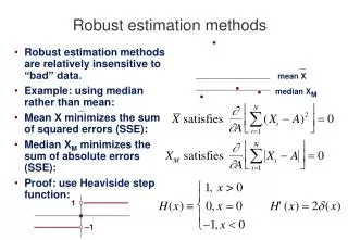
mean X Robust estimation methods • Robust estimation methods are relatively insensitive to “bad” data. • Example: using median rather than mean: • Mean X minimizes the sum of squared errors (SSE): • Median XM minimizes the sum of absolute errors (SSE): • Proof: use Heaviside step function: median XM 1 –1
How the median minimises SAE • Need to show that the median minimises the expected value of the sum of absolute errors: 0 (since X-XM=0 when H’ = 1 and H’=0 for all other values of X - XM)
Mean and median • The median is less sensitive to outliers than the mean. • Although the median is unbiased it is not a minimum-variance estimator. • Note how standard deviation of the median varies with sample size in comparison to standard deviation of the mean. Mean Median Median Mean
1 0 -1 Evaluation of median without sorting • A useful application:
Window Median filtering and sigma-clipping • Median filtering: take window of N points • Replace central point by median of the N points. • Sigma-clipping: • Fit all points by minimising 2 • Set threshold K and check for outliers at ± K or more • Repeat fit omitting largest outlier • Iterate until set of rejected points converges. Reject Reject
Using 2min to reject models • Suppose we fit M parameters to N data points: • We use N-M because an N - parameter fit should fit N points exactly. • If model is good, then the best-fit 2min should be:
x What if 2min is too high? • Several possibilities to consider: • Statistical fluke – use 2 distribution to estimate probability • Wrong model – use 2 distribution to reject model • Right model, but additional (nuisance) parameters not correctly chosen: • Error bars too small. Re-scale. • The third possibility adds a constant to 2min . • Can still use 2min +1 to set 1- confidence intervals on parameter values. x
2=1 2min N–M Diagnosis of 2min ≠ N-M ±√2(N-M) N–M 2= 2min /(N–M) >1 2= 2min /(N–M) < 1 2min N–M 2min > N–M due to under-estimation of error bars 2min > N–M due to unimportant parameters omitted from model 2min < N–M due to over-estimation of error bars If this happens use these values to estimate errors on parameters